Kill Time At Work With Recreational Math: Let's Simulate a Radioactive Sample

This is the 8^th in my series of killing time at work using math (the others are listed at the bottom of this post) and it's the first time that I have ever made an animated gif.

If you have read my posts before you already know that there are a few prerequisites for this:

• You like recreational math.
• You work at a computer and have access to Microsoft Excel.
• You are bored out of your tree.
• You don't want to get caught slacking off.

So, let's get started.

---

In this post we are going to simulate a sample of a radioactive isotope. The thing about radioactive substances is that you can never know when any individual atom is going to decay but if you have a large sample of these atoms then you can get a good idea of its half-life.

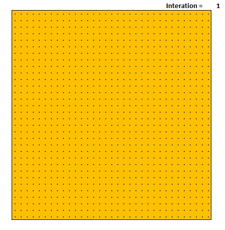
In the spreadsheet (see below) we are going to set up two grids, a 'pretty' one that simulates whether an atom has decayed or not and a second grid that counts how many atoms have not yet decayed.

The second grid will be used to help us to plot the decay curve and this will be useful to validate that our simulation is behaving in the same we that a radioactive sample would behave.

Excel Cell Updates Are Raster Scans

It is important to remember that Excel updates each cell using a raster scan technique. It starts at cell A1 and updates to the right in that row right to the end. It then goes to cell B1 and updates that row left-to-right. It does this all the way to the bottom of your spreadsheet.

Excel Calculation Options

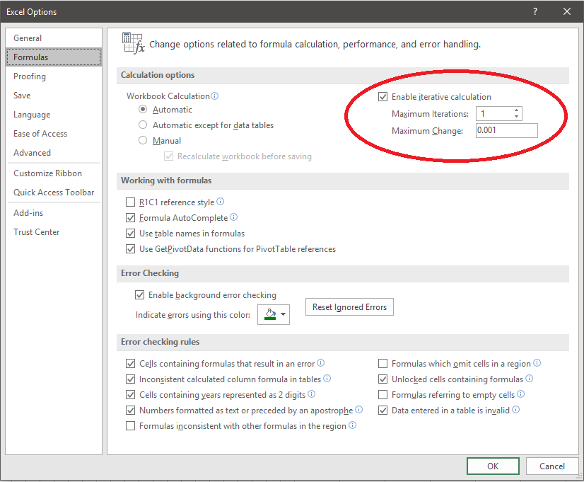
1. Go to the File tab in Excel and choose Options.
2. When the Options dialogue pops up choose Formulas.
3. The Dialogue for formula/calculation options will appear.
4. In this dialogue make sure you set the maximum number of iterations for calculations to 1 (circled in red). If you don't Excel will simply scream through all of the calculations and you will not see anything except for the final generation.

The Spreadsheet

I will now go through each cell and describe what it does.

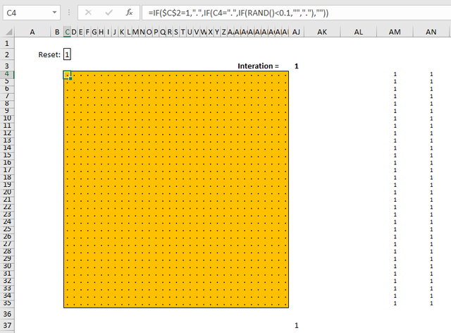
Cell C2: This is the reset cell. Set it to 1 and hit 'F9'to fill the grid back up with un-decayed atoms. Delete it and hit 'F9' to get the simulation to increment forward by one iteration. You must hit 'F9' each time you want a new iteration.

Cells C4 to AI35: =IF($C$2=1,".",IF(C4=".",IF(RAND()<0.1,"","."),""))

This cell first checks if the reset cell (Cell C$2 is set to 1. If it is then it will simply set the value of that cell to "." (this is a handy way to reset the entire grid).

If the reset cell has any other value than "." then it will instead execute this equation:
IF(C4=".",IF(RAND()<0.1,"","."),"")

If the cell is a "." character (i.e. it has not decayed yet) then execute the random function. If the random function returns a value less then 0.1 then set the cell to a blank character "". If the random function returns 0.1 or higher then leave it as a "." character.

If the cell is a "" character (i.e. it has decayed) then just leave it as an empty character.

Copy the equation =IF($C$2=1,".",IF(C4=".",IF(RAND()<0.1,"","."),"")) from C4 to AI35. The C4 reference in the equation is a relative reference and it will automatically update as you copy it down and across.

Cell AJ3: =IF(C2=1,1,IF(AJ3=AJ38,AJ3+1,AJ3))
This cell is not critical to the calculation. It just counts the number of iterations using the above equation.

There is a mirror cell (cell AJ38) that I use to copy the value of AJ3 in each iteration. Remember that Excel has no loop function so we need these tricks to simulate iterative activities within Excel.

Also remember that, as mentioned above, Excel updates cells in a raster scan fashion so the order in which you place your cells and columns matters.

b>Cell AJ38: =AJ3
This cell just copies the value of cell AJ3. Every time you hit F9 to trigger an iteration cells AJ3 and AJ38 will work together to count up from 1.

Validating The Simulation (Let's Plot The Decay Curve)

So you can stop there and just enjoy your radioactive sample simulation. That's really good enough but if you are curious about whether the 'atoms' in this simulation decay away in the expected manner it is good to plot out the remaining population of un-decayed atoms at each iteration.

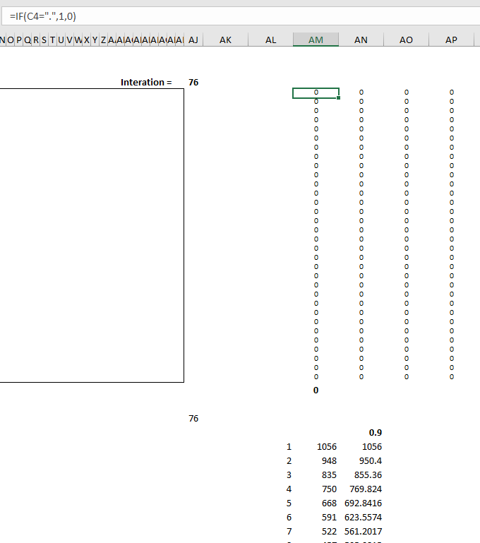
Cells AM4 to BS35: =IF(C4=".",1,0)
This is the secondary grid and its only purpose is to just count up the cells in the primary grid that are equal to ".". The formula checks if its companion cell in the primary grid is equal to "." and if so it will set the cell value to 1, otherwise it will set it to 0.

Cell AM36: =SUM(AM4:BS35)
This cell sums up the values in the entire secondary grid. This is how many 'atoms' have not decayed away yet.

Cells AL40 to AL140 The Plot Counter
This is the x-axis of the plot. This is just a column going from 1 to 100 and it will be used to help generate the plot.

Cells AM40 to AM140: =IF(AL40=AJ$3,AM$36,AM40)
This is the y-axis of the plot.

This column will check if the value of the counter cell (cell AJ$3) is equal to the value of the plot counter cell described above. If so then it will set its value to the summation cell (AM36, otherwise it will just leave it alone.

If all works well this setup will automatically update the proper y value in the x,y grid that can be used to plot the decay curve.

Column AN (Cells AN39 to AN140)
You can see that in this column I was just checking to see if my simulation decayed away as it should. I used a decay factor of 0.9 and the two curves seem to match up. This is encouraging and shows that I did not screw up.

The Result

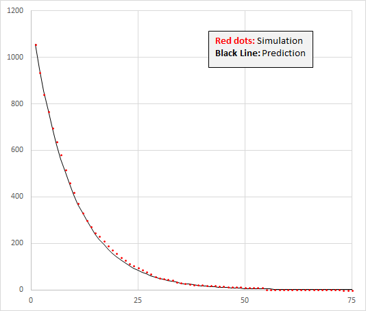
Here is a plot of the results. The red dots are the simulation results as a function of iteration. The y-axis is the number of atoms left and the x-axis is the time (iteration number). The black curve is the prediction. I set the simulation equation to be RAND() < 0.1 which means that each iteration about 90% of the total should remain.

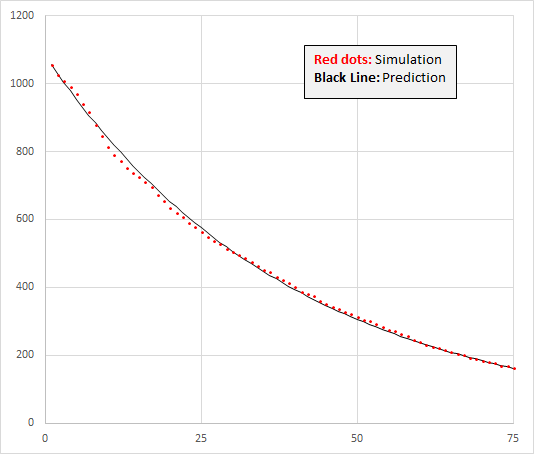
Here is the result when I set the simulation equation to be RAND() < 0.025. We get a less steep drop-off and the simulation data dances around the prediction line really nicely. It's a good illustration of how real world data is always rougher than the text book equations.

Closing Words

Overall the simulation appears to mimic a radioactive decay curve fairly accurately. It's not linear which is good and there is a good long tail as you would expect. You can also see that the curve is not smooth as would be expected if you had a sample size of just 1000 radioactive atoms. The decay rate is fast at first but as fewer and fewer atoms are left you will have to wait longer and longer periods between decay events.

If you like this then you may want to try to make a bigger grid to get a better sample size.

Also you may want to vary the "RAND() < 0.1" part of the function in cells C4 to AI35. Making it smaller than 0.1 will cause the it to decay more slowly (and vice versa).

In general this a good educational tool and should help you understand both the random nature of radioactive decay as well as the more predictable half-life decay constant that can be calculated from the random decay events of a large sample.

Thank you for reading my post.

Other Posts In My Recreational Math Series

1. Testing the excel random function.
2. Make Your Own Bell Curve
3. Strange Attractors.
4. Let's Travel To Alpha Centauri
5. Calculate Sunset and Sunrise Times
6. Conway's Game of Life.
7. Caffeine Half-Life.

Post Sources

[1] Half-Life Explained
[2] Microsoft Excel Wikipedia article
[3] Microsoft Excel Official Page
[4] The animated gif in this post was created using this website: https://ezgif.com/maker and by uploading 50 screenshots of my Excel grid.