#ulog (Tutorial @ 003)Unleashing the Capabilities of MATLAB #2 (Basic Signal Operations: Continuous-Time Signal)
Stop that gloomy face because today "WE ARE ABOUT TO LEARN MORE"
What is MATLAB?
![]()
MATLAB (matrix laboratory) is a multi-paradigm numerical computing environment. A proprietary programming language developed by MathWorks, MATLAB allows matrix manipulations, plotting of functions and data, implementation of algorithms, creation of user interfaces, and interfacing with programs written in other languages, including C, C++, C#, Java, Fortran and Python. ---Wikipedia
MATLAB is specifically designed for engineers and scientists. It possesses a matrix-based language that allows natural act or instance of representing a computational mathematics.
MATLAB combines a desktop environment tuned for iterative analysis and design processes with a programming language that expresses matrix and array mathematics directly.
A glimpse in the Capabilities of MATLAB
Click the words with the font color of green to be directed to some posts I’ve already exposed about MATLAB.
In the post above, you’ll be able to understand the big difference between a continuous-time signal and a discrete-time signal using MATLAB.
In the post above, you’ll be able to know how to INSTALL, ACTIVATE, and RUN MATLAB.
These days I am exploring more of this amazing and interesting application and as I am learning, I kind of wanting to share it to you so here I am. So, without further ado, this time, we are going to learn about the Basic Signal Operations of Digital Processing Signals
What are the Basic Signal Operations of Digital Processing Signals?
Time Shifting
Time Shifting Operation is the result you get when you change the positioning of the signal without affecting its amplitude. It can either be delayed or advanced compared to the original signal. To change the positioning of a signal you just need to subtract the fundamental period from the time.Time Reversal
Time Reversal Operation is basically the reflection or the reverse of the original signal. To reverse a signal, you just need to multiply time with negative one.Time Scaling
Time Scaling Operation is the result when the time of the original signal is being multiplied by a time-variable or a scaling factor. The original signal can either be stretched or compressed.
To understand more about the basic signal operations, let us construct codes that will show their graphs by using MATLAB.
Things to consider in using MATLAB
Put Two Percent-Signs (%%)
Always put two percent-signs to create sections of the program. This is necessary when we are dealing with various elements and codes that are meant for different graphs or commands. This allows us to run the program separately from other sections.MATLAB is Sequential Type of Programming Platform
This factor is very important to remember since the program may not be able to run if the inputted values are not in sequence. Therefore, there is a sequence that is in need to be followed. It is essential to first encode the values of every variables you are to represent before encoding a function or equation.Put Colon (:) to Create Matrix
Put colon whenever you want to construct a matrix. Let us use time as an example. Time is an independent variable and since it has no ending, for us to establish limits we need to construct a matrix. So, how to construct a matrix? Just follow start:interval:end.Variables Represented are Limited
The only variables that can be represented in a MATLAB are letters, numbers, and dollar sign.Parenthesis is in Need to Analyze the Program
When you are about to call or analyze the program you made, you need to enclose the Variable you represent with parenthesis.plot(variable represented)
That is what you need to encode when you are going to analyze a program for Continuous-Time Signal.stem(variable represented)
That is what you need to encode when you are going to analyze a program for Discrete-Time Signal.subplot(y,x,n)
To subplot programs, you need to consider the number of figures that are to be represented in y-axis, x-axis and the number of variables to be represented. y is for the number of figures that are to be represented in y-axis; x is for the number of figures that are to be represented in x-axis; and n is for the number of variables to be represented.
Sneak Peak for This Topic:
- Our original signal is the Continuous-Time Signal and we’ll have sinewave as an example since it is common and easy to understand. Sinewave is equal to
A*sin(2*pi*f*t)
- Since we have too many functions and sections to perform so you’ll also be learning how to save a function and how to call it.
This function will be used throughout the entire program
- When plotting a called function you must use
plot(*time*,*variable*);
We use xlabel('Your preferred name') to label every section.
Our fundamental periods are denoted with t0.
Our scaling factor is denoted with a.
We’ll be having seven sections in this program.
Using MATLAB
Open your MATLAB
Go to the MATLAB Editor to start encoding the program
First, we are going to apply the operations in Continuous-Time Signal. Then we are going to compare all graphs.
- The whole program will begin in creating a function. So, in the editor, type the codes I encoded below
function xt = sinewave(A,f,t)
xt = A*sin(2*pi*f*t)
end
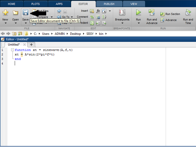
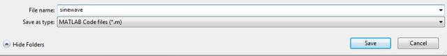
- Save it using ”sinewave”
- Open another Editor and let us start with our Original Signal
Since I stated above that sinewave is what we are going to use as an example, so we’ll first create our first section. This section will be our original signal.
%% Continuous
We are already aware that MATLAB is sequential, so we’ll input the important values that we need. But this time, since we are calling a function from the first editor then time will only be the value we need to be encoded first before encoding anything else in the program
t = [0:.001:.06];
Now let us encode the equation of the first variable we are to represent. And you may be curious about its structure but that is what our equations will look like because once again, we are calling the function we made in the first editor.
Y = sinewave(10,50,t);
Since the goal is to represent “Y” we’ll follow the rules above.
plot(t,Y);
To recognize the section, let us label it.
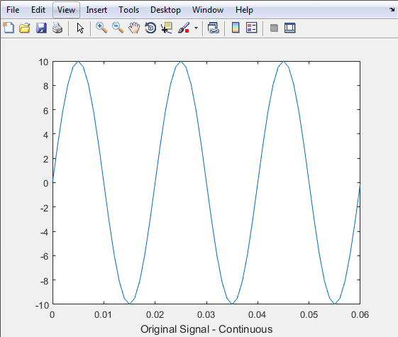
xlabel('Original Signal - Continuous')
So, the first section is:
%% Continuous
t = [0:.001:.06];
Y = sinewave(10,50,t);
plot(t,Y);
xlabel('Original Signal - Continuous')
Then press the "Run" icon to run the program.
The graph below is the representation of the Continuous-Time Signal we encoded.
- We’ll be having two Time Shifting Operations to show us the difference between ADVANCE and DELAY. These will serve as our second and third sections. Time Shifting results when we subtract periods (t0) from our time (t)
Starting with ADVANCE, we are going to provide another section.
%% Time Shifting: Advance
We are already aware that MATLAB is sequential, so we’ll input the important values that we need except for the values we already inputted in our original signal.
Signal is shifted to ADVANCE when the value of our (t0) is greater than zero.
t0 = 2;
Now let us encode the equation of the second variable we are to represent.
Y1 = sinewave(10,50,t-t0);
Since the goal is to represent “Y1” we’ll follow the rules above.
plot(t-t0,Y1);
To recognize the section, let us label it.
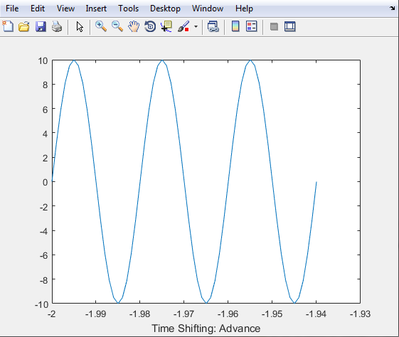
xlabel('Time Shifting: Advance')
So, the second section is:
%% Time Shifting: Advance
t0 = 2;
Y1 = sinewave(10,50,t-t0);
plot(t-t0,Y1);
xlabel('Time Shifting: Advance')
Then press the "Run" icon to run the program.
The graph below is the representation of the Continuous-Time Signal we encoded.
This time, we’ll be having the DELAY. We are going to provide another section.
%% Time Shifting: Delay
We are already aware that MATLAB is sequential, so we’ll input the important values that we need except for the values we already inputted in our original signal.
Signal is shifted to DELAY when the value of our (t0) is less than zero.
t0 = -2;
Now let us encode the equation of the third variable we are to represent.
Y2 = sinewave(10,50,t-t0);
Since the goal is to represent “Y2” we’ll follow the rules above.
plot(t-t0,Y2);
To recognize the section, let us label it.
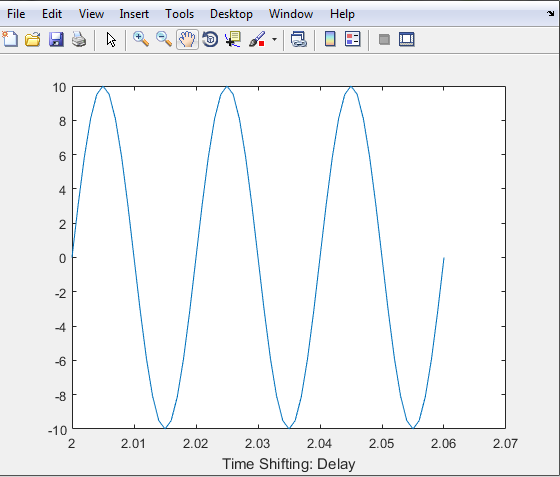
xlabel('Time Shifting: Delay')
So the third section is:
%% Time Shifting: Delay
t0 = -2;
Y2 = sinewave(10,50,t-t0);
plot(t-t0,Y2);
xlabel('Time Shifting: Delay')
Then press the "Run" icon to run the program.
The graph below is the representation of the Continuous-Time Signal we encoded.
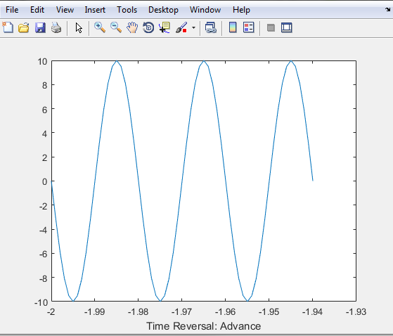
- We’ll be having two Time Reversal Operations to show us the difference between the Reversal of ADVANCE and the Reversal of DELAY. Time Reversal results when multiplying negative one (-1) to our time (t)
Starting with ADVANCE, we are going to provide another section.
%% Time Reversal: Advance
We are already aware that MATLAB is sequential, so we’ll input the important values that we need except for the values we already inputted in our original signal.
Signal is shifted to ADVANCE when the value of our (t0) is greater than zero.
t0 = 2;
Now let us encode the equation of the fourth variable we are to represent.
Y3 = sinewave(10,50,-1*t-t0);
Since the goal is to represent “Y3” we’ll follow the rules above.
plot(t-t0,Y3);
To recognize the section, let us label it.
xlabel('Time Reversal: Advance')
So the fourth section is:
%% Time Reversal: Advance
t0 = 2;
Y3 = sinewave(10,50,-1*t-t0);
plot(t-t0,Y3);
xlabel('Time Reversal: Advance')
Then press the "Run" icon to run the program.
The graph below is the representation of the Continuous-Time Signal we encoded.
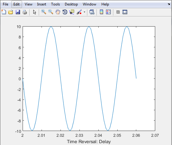
This time, we’ll be having the DELAY. We are going to provide another section.
%% Time Reversal: Delay
We are already aware that MATLAB is sequential, so we’ll input the important values that we need except for the values we already inputted in our original signal.
Signal is shifted to DELAY when the value of our (t0) is less than zero.
t0 = -2;
Now let us encode the equation of the fifth variable we are to represent.
Y4 = sinewave(10,50,-1*t-t0);
Since the goal is to represent “Y4” we’ll follow the rules above.
plot(t-t0,Y4);
To recognize the section, let us label it.
xlabel('Time Reversal: Delay')
So the fifth section is:
%% Time Reversal: Delay
t0 = -2;
Y4 = sinewave(10,50,-1*t-t0);
subplot(8,2,11);
plot(t-t0,Y4);
xlabel('Time Reversal: Delay')
Then press the "Run" icon to run the program.
The graph below is the representation of the Continuous-Time Signal we encoded.
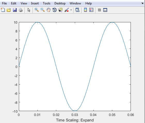
- We’ll be having two Time Scaling Operations to show us the difference between EXPANDED and COMPRESSED version of the Original Signal. Time Scaling results when we multiply a scaling factor (a) to our time (t)
Starting with EXPANDED; we are going to provide another section.
%% Time-Scaling: Expanded
We are already aware that MATLAB is sequential, so we’ll input the important values that we need except for the values we already inputted in our original signal.
Signal is scaled to EXPAND when the value of our (a) is greater than zero but less than 1.
a = .5;
Now let us encode the equation of the sixth variable we are to represent.
Y5 = sinewave(10,50,a*t);
Since the goal is to represent “Y5” we’ll follow the rules above.
plot(t,Y5);
To recognize the section, let us label it.
Xxabel('Time Scaling: Expanded');
So the sixth section is:
%% Time Scaling: Expand
a = .5;
t = [0:.001:.06];
Y5 = sinewave(10,50,a*t);
plot(t,Y5);
xlabel('Time Scaling: Expand')
Then press the "Run" icon to run the program.
The graph below is the representation of the Continuous-Time Signal we encoded.
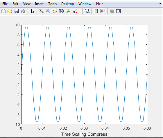
This time, we’ll be having the COMPRESSED version of the original signal. We are going to provide another section.
%% Time-Scaling: Compressed
We are already aware that MATLAB is sequential, so we’ll input the important values that we need except for the values we already inputted in our original signal.
Signal is scaled to COMPRESS; when the value of our (a) is greater than one.
a = 2;
Now let us encode the equation of the seventh variable we are to represent.
Y6 = sinewave(10,50,a*t);
Since the goal is to represent “Y6” we’ll follow the rules above.
plot(t,Y6);
To recognize the section, let us label it.
xlabel('Time Scaling: Compressed')
So the seventh section is:
%% Time Scaling: Compress
a = 2;
t = [0:.001:.06];
Y6 = sinewave(10,50,a*t);
plot(t,Y6);
xlabel('Time Scaling:Compress')
Then press the "Run" icon to run the program.
The graph below is the representation of the Continuous-Time Signal we encoded.
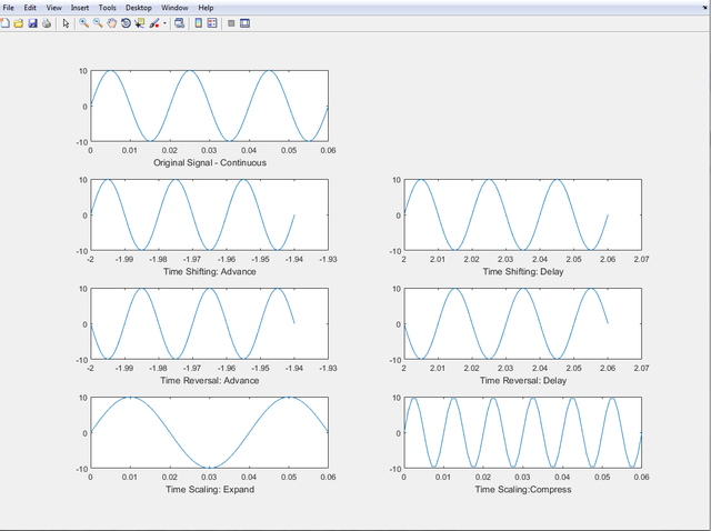
SUBPLOTTING
This time, we’ll be comparing the graph from each other to see their difference and to prove the validity of the operations. We are going to have 4 figures that are to be represented in y-axis; 2 figures that are to be represented in x-axis; and 7 represented variables.
Since “CONTINUOS-TIME SIGNAL” is our original signal then it’ll be our 1st n
%% Continuous
t = [0:.001:.06];
Y = sinewave(10,50,t);
subplot(4,2,1);
plot(t,Y);
xlabel('Original Signal - Continuous')
We are not going to put our 2nd n so that the only graph at the top is the original signal. And in that way we can compare them easily. The other variables we’ll encode will be simultaneous from the 3rd n till 8th.
%% Time Shifting: Advance
t0 = 2;
Y1 = sinewave(10,50,t-t0);
subplot(4,2,3);
plot(t-t0,Y1);
xlabel('Time Shifting: Advance')


%% Time Shifting: Delay
t0 = -2;
Y2 = sinewave(10,50,t-t0);
subplot(4,2,4);
plot(t-t0,Y2);
xlabel('Time Shifting: Delay')

%% Time Reversal: Advance
t0 = 2;
Y3 = sinewave(10,50,-1*t-t0);
subplot(4,2,5);
plot(t-t0,Y3);
xlabel('Time Reversal: Advance')

%% Time Reversal: Delay
t0 = -2;
Y4 = sinewave(10,50,-1*t-t0);
subplot(4,2,6);
plot(t-t0,Y4);
xlabel('Time Reversal: Delay')

%% Time Scaling: Expand
a = .5;
t = [0:.001:.06];
Y5 = sinewave(10,50,a*t);
subplot(4,2,7);
plot(t,Y5);
xlabel('Time Scaling: Expand')

%% Time Scaling: Compress
a = 2;
t = [0:.001:.06];
Y6 = sinewave(10,50,a*t);
subplot(4,2,8);
plot(t,Y6);
xlabel('Time Scaling:Compress')
The final program will be:
%% Continuous
t = [0:.001:.06];
Y = sinewave(10,50,t);
subplot(4,2,1);
plot(t,Y);
xlabel('Original Signal - Continuous')
%% Time Shifting: Advance
t0 = 2;
Y1 = sinewave(10,50,t-t0);
subplot(4,2,3);
plot(t-t0,Y1);
xlabel('Time Shifting: Advance')


%% Time Shifting: Delay
t0 = -2;
Y2 = sinewave(10,50,t-t0);
subplot(4,2,4);
plot(t-t0,Y2);
xlabel('Time Shifting: Delay')

%% Time Reversal: Advance
t0 = 2;
Y3 = sinewave(10,50,-1*t-t0);
subplot(4,2,5);
plot(t-t0,Y3);
xlabel('Time Reversal: Advance')

%% Time Reversal: Delay
t0 = -2;
Y4 = sinewave(10,50,-1*t-t0);
subplot(4,2,6);
plot(t-t0,Y4);
xlabel('Time Reversal: Delay')

%% Time Scaling: Expand
a = .5;
t = [0:.001:.06];
Y5 = sinewave(10,50,a*t);
subplot(4,2,7);
plot(t,Y5);
xlabel('Time Scaling: Expand')

%% Time Scaling: Compress
a = 2;
t = [0:.001:.06];
Y6 = sinewave(10,50,a*t);
subplot(4,2,8);
plot(t,Y6);
xlabel('Time Scaling:Compress')
See the difference for yourself:
References
- CTandDT - Digital Signal Processing by Engineer Junard Kaquilala
Go here https://steemit.com/@a-a-a to get your post resteemed to over 72,000 followers.
Hi! This is jlk.news intelligent bot. I just upvoted your post based on my criteria for quality. Keep on writing nice posts on Steemit and follow me @jlkreiss to get premium world news updates round the clock! 🦄🦄🦄
Nosebleed lol! I checked your profile and no wonder you are writing such topic. I learned something today but it's all jargon. This needs re-reading and further reading about the topic.
...i was glad you are studying BSECE...good job kabayan