[머신러닝] MNIST Data로 숫자 이미지 분류하기
MNIST Data
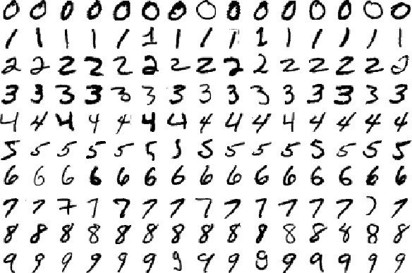
그동안 우리가 학습한 내용을 활용해서 이미지 분류 작업을 할 수 있다. 위의 그림과 같이 여러 사람이 다양한 형태로 표기한 숫자 이미지 파일을 픽섹 단위로 분해해서 학습할 수 있다는 의미다. 임의의 새로운 숫자 이미지 파일이 들어와도 어떤 숫자인지 분류하기 위한 목적이다.
import tensorflow as tf
from tensorflow.examples.tutorials.mnist import input_data
# Check out https://www.tensorflow.org/get_started/minist/beginners
# for more information about the mnist dataset
mnist = input_data.read_data_sets('MNIST_data/', one_hot=True)

nb_classes = 10
TensorFlow에서 예시로 제공해주는 데이터가 이미 있으므로 이를 활용해서 연습할 수 있다. tensorflow.example.tutorials.mnist 라이브러리에서 input_data를 가져온 후 MNIST_data를 읽어온다. 이때 one_hot을 True로 설정해두면 우리가 따로 작업하지 않아도 결과 데이터를 one-hot-encoding 형태로 가져올 수 있다. 우리가 분류하기 원하는 총 결과값은 0 ~ 9까지 총 10개의 label이다.
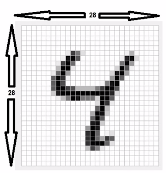
우리가 분석해야 할 X 값은 위 그림과 같이 가로 세로 28 * 28의 총 784개 픽셀이다. 그동안 10여 개의 feature를 학습했던 것보다 훨씬 많은 수의 학습이 이루어진다. feature의 개수와 결과값 Y의 label 개수를 고려해 아래의 코드와 같이 차원을 설정한다.
# MNIST data image of shape 28 * 28 = 784
X = tf.placeholder(tf.float32, [None, 784])
# 0 ~ 9 digit recognition = 10 classes
Y = tf.placeholder(tf.float32, [None, nb_classes])

W = tf.Variable(tf.random_normal([784, nb_classes]))
b = tf.Variable(tf.random_normal([nb_classes]))
특정 숫자로 제한된 결과값을 도출하기 위한 학습이기 때문에 softmax classification을 사용할 것이다. 앞서 배웠던 내용과 동일하다.
# Hypothesis (using softmax)
hypothesis = tf.nn.softmax(tf.matmul(X, W) + b)

cost = tf.reduce_mean(-tf.reduce_sum(Y * tf.log(hypothesis), axis=1))
optimizer = tf.train.GradientDescentOptimizer(learning_rate=0.1).minimize(cost)

# Test Model
is_correct = tf.equal(tf.argmax(hypothesis, 1), tf.argmax(Y, 1))
# Calculate Accuracy
accuracy = tf.reduce_mean(tf.cast(is_correct, tf.float32))
여기서 한 가지 이슈가 발생한다. TensorFlow에서 제공하는 train_data의 개수는 55,000개다. 전체 데이터를 한 번에 학습시키기에는 메모리가 부족하거나 과부하가 걸릴 수 있다. 이를 해결하기 위해 여러개의 batch로 나누어 여러번 학습을 진행하는 것이 효율적이다. batch는 전체 데이터 중 몇 개의 덩어리로 나눈 개념으로 이해하면 된다.
# parameters
training_epochs = 15
batch_size = 100

with tf.Session() as sess:
    # Initialize Tensorflow Variables
    sess.run(tf.global_variables_initializer())
    # Training cycle
    for epoch in range(training_epochs):
        avg_cost = 0
        total_batch = int(mnist.train.num_examples / batch_size)

        for i in range(total_batch):
            batch_xs, batch_ys = mnist.train.next_batch(batch_size)
            c, _ = sess.run([cost, optimizer], feed_dict={X: batch_xs, Y: batch_ys})
            avg_cost += c / total_batch

        print('Epoch: ', '%04d' % (epoch + 1), 'Cost: ', '{:.9f}'.format(avg_cost))
epoch이라는 개념도 나온다. 전체 55,000개 데이터를 한번씩 모두 학습하면 1 epoch이 된다. 위 코드에서 우리는 training_epochs=15로 설정했으므로 전체 55,000개 데이터를 15번, 즉 55,000 * 15 = 825,000개 데이터를 학습하게 된다.
training_epochs = 15을 반복하는 for loop 안에 전체 55,000개 데이터를 batch_size = 100으로 나눈 550번 반복해서 학습을 진행하는 for loop이 포함되어 있다. 각 epoch마다 cost를 계산할 수 있다.
Epoch:  0001 Cost:  2.817744847
Epoch:  0002 Cost:  1.090436493
Epoch:  0003 Cost:  0.863765682
Epoch:  0004 Cost:  0.753992744
Epoch:  0005 Cost:  0.685377607
Epoch:  0006 Cost:  0.637151059
Epoch:  0007 Cost:  0.600648493
Epoch:  0008 Cost:  0.571259752
Epoch:  0009 Cost:  0.547828114
Epoch:  0010 Cost:  0.528008322
Epoch:  0011 Cost:  0.510270363
Epoch:  0012 Cost:  0.496145278
Epoch:  0013 Cost:  0.482756565
Epoch:  0014 Cost:  0.471168885
Epoch:  0015 Cost:  0.460864195
학습이 진행될수록 cost가 감소하는 것을 확인할 수 있다.
# Test the model using test sets
    print('Accuracy: ', accuracy.eval(session=sess, feed_dict={X: mnist.test.images, Y: mnist.test.labels}))
마찬가지로 학습 모델의 최종적인 Accuracy도 계산할 수 있다. 참고로 sess.run이 아닌 함수명.eval(session=sess,...)로도 세션을 실행할 수 있다. 간단한 tensor를 실행시킬 때 사용할 수 있는 방법이다.
Accuracy: 0.8901
89.01%의 정확도를 보인다. 뛰어나다고는 할 수 없지만 간단한 코드 몇줄로 효과적인 학습을 진행했다고 볼 수 있다.
import matplotlib.pyplot as plt
import random

# Get one and predict
    r = random.randint(0, mnist.test.num_examples - 1)
    print('Label: ', sess.run(tf.argmax(mnist.test.labels[r:r+1], 1)))
    print('Prediction: ', sess.run (tf.argmax(hypothesis, 1), feed_dict={X: mnist.test.images[r:r+1]}))

    plt.imshow(mnist.test.images[r:r+1].reshape(28, 28), cmap='Greys', interpolation='nearest')
    plt.show()
실제로 우리의 학습이 잘 이루어졌는지 test_data를 활용해 검증해보자. 전체 test 데이터 중에서 하나의 숫자를 임의로 뽑아낸다. 해당 label이 우리가 가설로 세워 도출한 예측값과 실제로 일치하는지 비교해본다.
더불어 matplot 라이브러리를 사용해 해당 이미지 값을 나타내보자.
Label:  [4]
Prediction:  [4]
위와 같이 Label : 4에 대해 우리의 학습 예측값도 Prediction : 4로 일치됐다.

pairplay 가 kr-dev 컨텐츠를 응원합니다! :)
5월 다시 파이팅해요!
호출에 감사드립니다!