2-19 Iris flower data를 이용한 Rosenblatt 퍼셉트론 파이선 코딩(완결)

퍼셉트론 알고리듬에 따라 파이선으로 퍼셉트론 클라스 코딩을 해보자.
⓵ 퍼셉트론 클라스에 필요한 기본적인 파라메터로서 3가지 즉 learning rate, 학습횟수 및 랜덤 수 생성을 위한 seed 수를 준비하자.
class 코드에 처음에 eta 값이 0.01 로 지정되어 있지만 메인 코드에서 instance 값으로 0.1 을 부여하게 되면 부여된 instance에 맞춰 class 내 self에 의해서 self.eta 값이 0.1로 변환된다.
마찬가지로 학습 횟수에 해당하는 n_ier를 class 코드에 처음에는 50 으로 두지만 instance 값으로 10의 값을 주면 self에 의해서 self.n_iter 값이 10으로 변환된다.
seed 값을 예를 두어 1 로 두면 이 값이 바뀌지 않는한 항상 동일한 랜덤 수를 생성하여 연산하므로 동일한 결과를 얻어 볼 수 있다.

⓶ 퍼셉트론 클라스에서 필요한 속성(Attribute)으로서 입력 벡터 성분 웨이팅을 위한 1차원 어레이 w_ 와 지정된 학습횟수 내의 특정 에포크(epoch) 단계에서 전체 샘플들을 대상으로 생성되는 0.0이 아닌 업데이트 값들을 합하여 저장해 둘 리스트 즉 errors_를 1개 준비한다.
이 코드에서 보고자하는 중점 사항이 얼마나 빨리 업데이트(update) 값들의 합이 0.0에 수렴하느냐는 것이기 때문이다. 대체로 3∼6회에 0.0에 도달한다.
errors += int(update != 0.0)
업데이트 값의 정수만을 취하도록 되어 있는데 실수형(float) 로 바꿔도 큰 변화가 없다.

⓷ 아래에 퍼셉트론 class 파이선 코드를 참조하자.

class Perceptron(object):
"""Perceptron classifier.
Parameters
------------
eta : float (실수 learning rate, 0.0 과 1.0 사이)
n_iter : int (정수, 학습 횟수)
random_state : int (랜덤 수 생성을 위한 정수형 seed 값)

Attributes (속성)
-----------
w_ : 1d-array ( 1차원 어레이)
  Weights after fitting.
errors_ : list (리스트 데이터)
  Number of misclassifications (updates) in each epoch.

"""
def __init__(self, eta=0.01, n_iter=50, random_state=1):
    self.eta = eta
    self.n_iter = n_iter
    self.random_state = random_state

def fit(self, X, y):
    """Fit training data.

    Parameters
    ----------
    X : {array-like}, shape = [n_samples, n_features] (샘플수, 피처 수)
      Training vectors, where n_samples is the number of samples and
      n_features is the number of features.
    y : array-like, shape = [n_samples]
      Target values.(학습을 위한 라벨 값)

    Returns
    -------
    self : object

    """
    rgen = np.random.RandomState(self.random_state)
    self.w_ = rgen.normal(loc=0.0, scale=0.01, size=1 + X.shape[1])
    self.errors_ = []

    for _ in range(self.n_iter):
        errors = 0
        for xi, target in zip(X, y):
            update = self.eta * (target - self.predict(xi))
            self.w_[1:] += update * xi
            self.w_[0] += update
            errors += int(update != 0.0)
        self.errors_.append(errors)
    return self

def net_input(self, X):
    """Calculate net input"""
    return np.dot(X, self.w_[1:]) + self.w_[0]

def predict(self, X):
    """Return class label after unit step"""
    return np.where(self.net_input(X) >= 0.0, 1, -1)

⓸ class Perceptron(object) 의 코드 상 위치는 필요로 하는 라이브러리 모듈들을 import 한 다음이 헤더 영역이 좋을 것이다.

⓹지정된 서버 주소로부터 저장되어 있는 Iris data 세트를 읽어오자. 이 명령들이 셸(Shell)에서 실행되면 df.tail() 명령에 의해 끝 자락의 몇 줄 데이터를 출력해 주지만 파이선 편집기 내부 코드로 실행되면 df.tail() 결과를 볼 수 없음에 유의하자. 아무런 출력이 없다는 것은 제대로 실행이 잘된다는 의미이다.

df = pd.read_csv('https://archive.ics.uci.edu/ml/'
'machine-learning-databases/iris/iris.data', header=None)
df.tail()

⓺ 다시 한번 데이터를 읽어 오는 작업인데 이 내용은 현재 실행하는 파이선 코드 저장 위치와 읽어 온 Irsis-flower data set 저장 위치를 동일하게 해주는 역할이다.

df = pd.read_csv('iris.data', header=None)
df.tail()

⓻ 머신 러닝 작업을 하기 전에 Iris 데이터를 작도해 보자.
setosa 와 versicolor 2 종류의 붓꽃 데이터를 불러오자.
df.iloc[0:100, 4].values 는 150개로 구성되는 Iris 데이터에서 0번에서 99번까지 100개의 데이터 중 마지막 4번째 줄 데이타를 불러와 출력한다는 뜻이다.
Iris data 는 꽃 하나 당 0∼3번에 해당하는 4개의 실수형 숫자 데이터와 마지막 4번에 해당하는 문자열 꽃 이름으로 구성된다. 4개의 실수 데이터는 각각 꽃받침 길이와 폭 그리고 꽃잎의 길이와 폭 데이터로 구성된다.
불려온 데이터는 np.where() 명령에 의해서 ‘Iris-setosa’인지 확인 후 사실이면 라벨 값 –1을 부여하고 아니면 +1 값을 부여한다. 50개만 Iris-setosa 이므로 –1 데이터 및 +1 데이터가 각각 50개씩 생성된다.

y = df.iloc[0:100, 4].values
y = np.where(y == 'Iris-setosa', -1, 1)

⓼꽃받침과 꼬치잎의 길이 데이터만 가지고도 setosa 와 versicolor 종을 쉽게 구별할 수 있으므로 이 2종류의 데이터를 가지고 입력 벡터 데이터들의 샘플을 준비하자.
#extract sepal(꽃받침) length and petal(꽃잎) length

X = df.iloc[0:100, [0, 2]].values

⓽ 2종류의 붓꽃 데이터를 가로축은 꽃받침 길이 세로축은 꽃잎 길이로 하여 작도하자.

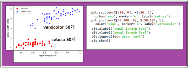
⓾ 2개의 좌표 즉 (꽃받침 길이, 꽃잎 길이)로 구성되는 붓꽃 데이터를 학습 시키자. 즉 이 좌표 데이터에 원래 데이터에서 매겨져 있던 타겟 라벨값 “+1” 또는 “-1” 이 되도록 지속적으로 웨이트 값을 업데이트하자. 각 데이터 합(∑,시그마)을 계산하여 그 부호가 +이면 “+1” 값을 – 이면 “-1” 값을 부여하는데 타겟 라벨 값과 같아지면 더 이상 업데이트 할 필요가 없으며 그 데이터는 학습이 끝난 것이다. 즉 그 데이터의 적절한 웨이트 값이 선정된 것이다.
대부분의 데이터들이 1∼2회에 학습이 완료되며 나머지 아주 소수의 데이터들이 3∼5회면 거의 끝난다.
ppn = Perceptron(eta=0.1, n_iter=10) ( learning rate = 0.1, 학습횟수를 10으로 하여
class Perceptron 실행에 의해 instance ppn을 생성한다)
ppn.fit(X, y) (입력 벡터 X 와 타겟 라벨 값 y를 사용하여 class perceptron 내부의
fit 함수에 의해서 학습을 시킨다)
plt.plot(range(1, len(ppn.errors_) + 1), ppn.errors_, marker='o') ( 에러의 합을 계산해 두었다가 학습횟수 증가에 해당하는 에포크(epoch) 별로 그 값을 그래프로 출력한다)
plt.xlabel('Epochs')
plt.ylabel('Number of updates')
plt.show()

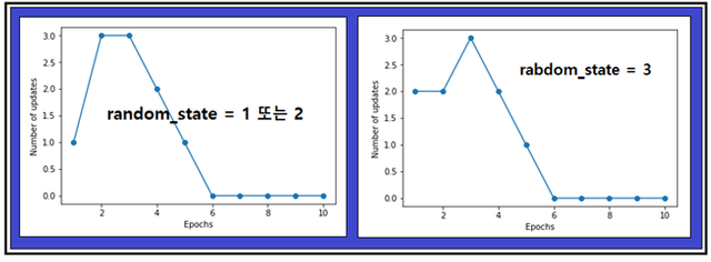
랜덤 수의 초기 값에 해당하는 random_state 값이 1 또는 2일 때와 3일 때의 두가지 경우가 출력되는데 워낙 간단한 문제라 계속 바꿔 봐도 둘 중의 하나가 출력된다. 5회까지 웨이트를 업데이트 하면 100개의 데이터 학습이 완료됨을 알 수 있다.

여기까지가 위 스캐터 플롯에서 보듯이 두 무더기로 이루어지는 Iris flower data set 100개를 대상으로 한 학습 과정이라면 두 무더기 데이터들을 구별할 수 있도록 쉽게 직선을 그을 수 있으며 이러한 특성을 “선형적으로 구분 가능하다“ 또는 원어로 ”linearly separable“하다고 정의 한다.

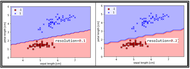
선형구분선은 임의로 보고 긋는 것이 아니며 설정된 가로축과 세로축 공간에서 범위를 정해 눈금을 생성하면 눈금 좌표들이 생성되는데 이들 좌표들을 학습시켜야 할 필요가 있다. 즉 학습이 되면 전체 눈금들에 대해 “+1” 인지 “-1”인지 라벨 값이 결정이 되는데 이 값들을 이용하여 contour를 작도하면 contour 레벨 값에 해당하게 되는 색상 속성이 부여된 라벨 값들이 딱 2가지뿐이므로 색상이 불연속적이 되는 경계선을 시각적으로 볼 수 있으며 이 경계선을 decision boundary 라고 한다.

⑪ decision boundary를 작도하기 위한 함수를 구성해 보자. X 는 입력 벡터이며 y는 입력 벡터에 대응하는 라벨 값이다. classifier는 미리 앞에서 선언해둔 class Perceptron을 불러필요 시 instance를 생성하도록 한다. 해상도는 눈금 데이터 생성 시 해상도 간격을 뜻한다.
다음 그림에서 보면 해상도 간격이 커질수록 decision boundary 가 엉성해 짐을 볼 수 있다.

def plot_decision_regions(X, y, classifier, resolution=0.02):
# setup marker generator and color map
markers = ('s', 'x', 'o', '^', 'v')
colors = ('red', 'blue', 'lightgreen', 'gray', 'cyan')
cmap = ListedColormap(colors[:len(np.unique(y))]) ( unique(y) 값이 “+1” 과
“-1” 두가지이므로 ‘red’ 와 ‘blue’ 색상만 컬러맵 작성에 사용된다.
x1_min, x1_max = X[:, 0].min() - 1, X[:, 0].max() + 1 (가로축 데이터 범위에
각각 1만큼씩 양쪽으로 여유를 준다)
x2_min, x2_max = X[:, 1].min() - 1, X[:, 1].max() + 1 (세로축 데이터 범위에
각각 1만큼씩 아래 위 양쪽으로 여유를 준다)
xx1, xx2 = np.meshgrid(np.arange(x1_min, x1_max, resolution),
np.arange(x2_min, x2_max, resolution))
앞서 설정한 범위 내에서 해상도를 0.02 단위로 하여 세밀한 눈금 좌표를 생성한다.
눈금 좌표들은 가로축 xx1 좌표 어레이와 세로축 xx2 좌표 어레이의 합성으로 구성되며
이들을 뜯어내 각각 한 줄짜리 어레이로 구성( flatenning process) 후 Transpose 형태를 취하자. 이어서 class Perceptron을 의미하는 classifier를 불러 instance를 생성시키는 과정에서 눈금 데이터 xx1과 xx2 를 사용하여 클라스 내부에 정의된 함수 predict를 불러 학습을 시킨다.
Z = classifier.predict(np.array([xx1.ravel(), xx2.ravel()]).T)
Z = Z.reshape(xx1.shape ) (가로축 1차원 데이터 어레이 xx1.shape 하나만을 reshape
하면 원래대로 원상 복구된다.)
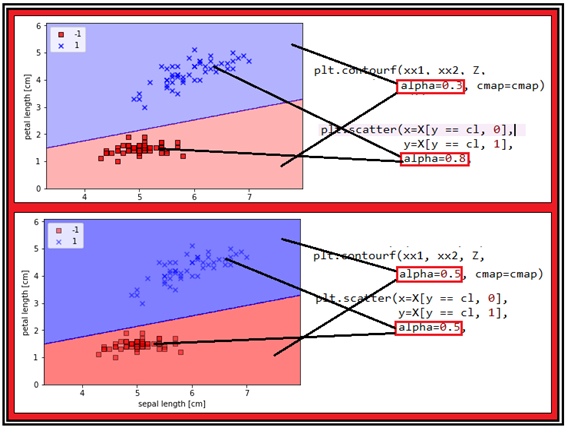
plt.contourf(xx1, xx2, Z, alpha=0.3, cmap=cmap) ( 학습된 Z는 색상 레벨 값 데이터 를 가지고 있어 레벨 별 컬러로 표현이 된다. alpha는 색상의 진한 정도dlek.)
plt.xlim(xx1.min(), xx1.max())
plt.ylim(xx2.min(), xx2.max())

decison boundary 로 분할되는 영역 설정 및 contour 작도를 위한 함수가 설정되었으면 눈금 데이터 contour 색상 작도에 중첩하여 matplotlib 라이브러리 모듈 명령을 사용하여 Iris flower data set을 scatter 형으로 함께 작도 하자.
#plot class samples
for idx, cl in enumerate(np.unique(y)):
plt.scatter(x=X[y == cl, 0],
y=X[y == cl, 1],
alpha=0.8,
c=colors[idx],
marker=markers[idx],
label=cl,
edgecolor='black')
이어서 decision boundary를 포함하는 각 영역을 색상을 부여하여 작도한다.
plot_decision_regions(X, y, classifier=ppn)
plt.xlabel('sepal length [cm]')
plt.ylabel('petal length [cm]')
plt.legend(loc='upper left')
plt.show()

이 코드 전체를 실행하면 Rosenblatt이 뉴론에 대해서 관찰하고 모델링했던 방식으로 입력 벡터들의 웨이팅 된 합(∑,시그마)을 계산 후 웨이트 업데이터 과정에 따라 학습을 완료하여 선형적으로 구분 가능한 decision bounday를 포함한 공간을 컬러풀하게 시각화하여 보여주게 된다.

TensorFlow가 설치된 윈도우즈 10 아나콘다 스파이더에서 아래의 파이선 코드를 다운 받아 실행해 보자.

#ch02_data_read_plot_1_2.py
import numpy as np
import pandas as pd
import matplotlib.pyplot as plt
from matplotlib.colors import ListedColormap

class Perceptron(object):
"""Perceptron classifier.

Parameters
------------
eta : float
  Learning rate (between 0.0 and 1.0)
n_iter : int
  Passes over the training dataset.
random_state : int
  Random number generator seed for random weight
  initialization.

Attributes
-----------
w_ : 1d-array
  Weights after fitting.
errors_ : list
  Number of misclassifications (updates) in each epoch.

"""
def __init__(self, eta=0.01, n_iter=50, random_state=1):
    self.eta = eta
    self.n_iter = n_iter
    self.random_state = random_state

def fit(self, X, y):
    """Fit training data.

    Parameters
    ----------
    X : {array-like}, shape = [n_samples, n_features]
      Training vectors, where n_samples is the number of samples and
      n_features is the number of features.
    y : array-like, shape = [n_samples]
      Target values.

    Returns
    -------
    self : object

    """
    rgen = np.random.RandomState(self.random_state)
    self.w_ = rgen.normal(loc=0.0, scale=0.01, size=1 + X.shape[1])
    self.errors_ = []

    for _ in range(self.n_iter):
        errors = 0
        for xi, target in zip(X, y):
            update = self.eta * (target - self.predict(xi))
            self.w_[1:] += update * xi
            self.w_[0] += update
            errors += int(update != 0.0)
        self.errors_.append(errors)
    return self

def net_input(self, X):
    """Calculate net input"""
    return np.dot(X, self.w_[1:]) + self.w_[0]

def predict(self, X):
    """Return class label after unit step"""
    return np.where(self.net_input(X) >= 0.0, 1, -1)

###Training a perceptron model on the Iris dataset

df = pd.read_csv('https://archive.ics.uci.edu/ml/'
'machine-learning-databases/iris/iris.data', header=None)
df.tail()

#..
df = pd.read_csv('iris.data', header=None)
df.tail()

####Plotting the Iris data
#select setosa and versicolor
y = df.iloc[0:100, 4].values
y = np.where(y == 'Iris-setosa', -1, 1)

#extract sepal length and petal length
X = df.iloc[0:100, [0, 2]].values

#plot data
plt.scatter(X[:50, 0], X[:50, 1],
color='red', marker='o', label='setosa')
plt.scatter(X[50:100, 0], X[50:100, 1],
color='blue', marker='x', label='versicolor')

plt.xlabel('sepal length [cm]')
plt.ylabel('petal length [cm]')
plt.legend(loc='upper left')

#plt.savefig('images/02_06.png', dpi=300)
plt.show()

####Training the perceptron model

ppn = Perceptron(eta=0.1, n_iter=10)
ppn.fit(X, y)

plt.plot(range(1, len(ppn.errors_) + 1), ppn.errors_, marker='o')
plt.xlabel('Epochs')
plt.ylabel('Number of updates')

plt.show()

####A function for plotting decision regions
def plot_decision_regions(X, y, classifier, resolution=0.1):

#setup marker generator and color map
markers = ('s', 'x', 'o', '^', 'v')
colors = ('red', 'blue', 'lightgreen', 'gray', 'cyan')
cmap = ListedColormap(colors[:len(np.unique(y))])

#plot the decision surface
x1_min, x1_max = X[:, 0].min() - 1, X[:, 0].max() + 1
x2_min, x2_max = X[:, 1].min() - 1, X[:, 1].max() + 1
xx1, xx2 = np.meshgrid(np.arange(x1_min, x1_max, resolution),
                       np.arange(x2_min, x2_max, resolution))
Z = classifier.predict(np.array([xx1.ravel(), xx2.ravel()]).T)
Z = Z.reshape(xx1.shape )
plt.contourf(xx1, xx2, Z, alpha=0.3, cmap=cmap)
plt.xlim(xx1.min(), xx1.max())
plt.ylim(xx2.min(), xx2.max())

#plot class samples
for idx, cl in enumerate(np.unique(y)):
    plt.scatter(x=X[y == cl, 0], 
                y=X[y == cl, 1],
                alpha=0.8, 
                c=colors[idx],
                marker=markers[idx], 
                label=cl, 
                edgecolor='black')

plot_decision_regions(X, y, classifier=ppn)
plt.xlabel('sepal length [cm]')
plt.ylabel('petal length [cm]')
plt.legend(loc='upper left')

plt.show()