In the previous chapter, the introduction gave a good insight into the Physics behind the experiment. This chapter will delve into the experimental techniques carried out in the experiment. This includes the apparatus used as well as how they were used.

3 - Experimental Techniques

In this experiment, a dip-probe, holding a thermometer and the sample, was progressively ‘dipped’ into a liquid Helium tank, until the sample was fully submerged in the liquid Helium. This allowed for the sample to be exposed to a temperature range of around 300K to 4.2K. As the probe was dipped, the software triggered the equipment to automatically take regular and frequent measurements of the resistance of the sample and its corresponding temperature, at each given time. Before starting the experiment, some configuring was necessary to allow for the equipment to operate as required. Figure 4 shows the apparatus.

Figure 4: Image showing the main apparatus of the experiment

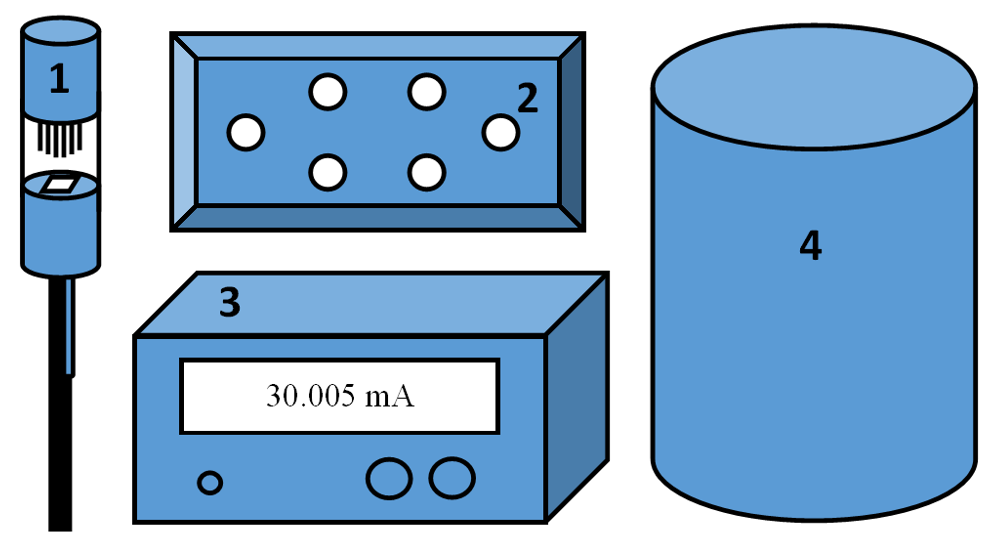
1. Probe-stick (themometer attached on rod below sample holder)
2. Breakout box (connects to pins on probe-stick)
3. Current source
4. Liquid helium container

3.1 - Testing the Sample Holder

The section of the dip-probe that held the sample consisted of 6 pins that were raised and lowered to remove and secure a sample in place. In this experiment, only 4 of the 6 are programmed to be used. These pins were cushioned by springs to stop the springs from breaking if lowered too fast or too hard. The pins are used to drive a current through the sample and allow for measurements to be taken, so they must be tested, before use, to make sure they work.

Figure 5: Image showing the pins on the probe-stick

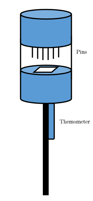
To test each individual pin, a multimeter is set to its ‘buzzer’ option; from then on, each port on the breakout box is connected to the multimeter with a probe, and the other probe is connected from the multimeter to the port’s corresponding pin on the dip-probe. A beep sounded on the multimeter for each pin, meaning that a current was passing through, meaning they were all functional. Despite the pins working, the springs were also tested to ensure the readings taken for the sample are reliable. To be able to test the springs, the structure of the probe-stick must be examined.

Figure 6: Image showing how the springs cushion the pin to help prevent it from breaking

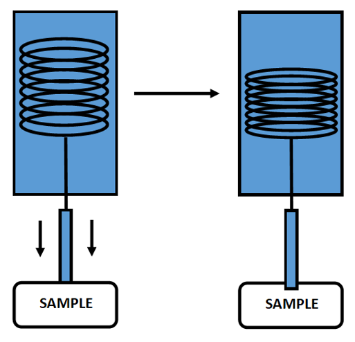
Figure 6 shows that the springs above the pins are submerged in the copper head of the probe-stick. This makes it considerably easy to test them. Again, a multimeter is set to ’buzzer’ and a probe is pressed and held against the copper head that contains the springs. Whilst holding the probe on the copper, the other probe is then inserted into each individual port on the breakout box. If a beep sounded from each port, all the springs worked; which they did.

3.2 - Configuring the Current Source

The current source is the piece of equipment that provides a current and measures the corresponding voltage of a sample. The reason the current source must be configured, is to allow it to work for the specific equipment used, in this experiment.

3.2.1 - Current Source settings

The configuration menu of the current source is accessed in order to alter some of the settings. The settings to be changed are as follows:

• Source is set to manual: this allows the user to change the current manually rather than automatically. This allows for more flexibility.
• Sense mode is set to 4-wire: since the experiment requires 4 pins out of the 6 to be used, setting the sense mode to 4-wire is a necessity, otherwise, the equipment will not be compatible.
• Offset is set to enabled; setting this option to enabled allows the equipment to attempt to eliminate thermal EMF, which is very important since the equipment is temperature dependant. Failure to get rid of this thermal EMF could contribute to a large experimental uncertainty.

Another benefit of configuring the current source this way, is that it can be used if the software fails to work at any point during the experiment. If this was to occur, measurements could then be taken manually to compensate for the faulty software. Having configured the current source, the sample is ready to be placed onto the probe stick.
Placing the Sample onto the probe-stick

3.3 - Placing the Sample onto the probe-stick

With the use of tweezers, to avoid contamination, the sample is placed on the slide, such that its surface lies directly under the pins. The pins on the probe-stick are then lowered slowly. As soon as the pins touch the sample, the current source shows a lot of fluctuations in the voltage. This fluctuation must be minimized, which is done by slowly lowering the pins even further. Lowering too much, or too fast, will damage the springs holding the pins, so this step is approached with great caution.

3.3.1 Choosing the optimum current for the sample

With the sample in place, an optimum current must be chosen to drive into the sample, to begin the experiment. Choosing the right current is essential to obtain the best signal-to-noise ratio. This is achieved by taking voltage measurements from a current range of 0.5mA to 60mA. Once measurements are taken, an IV characteristic is plotted. A current that lies on the straight-line section of the graph, where I∝V, is the optimum current to use for the experiment. The straight-line section of the graph is the Ohmic part of the graph as it obeys Ohm’s law, V∝I.

3.4 - Configuring the software

Once a suitable current has been chosen, the software takes over. Before the software can be used, it must again be configured to the equipment used in the experiment. When configured correctly, IV characteristics and resistance-temperature relations can be plotted. Time/ s

3.4.1 - IV characteristics

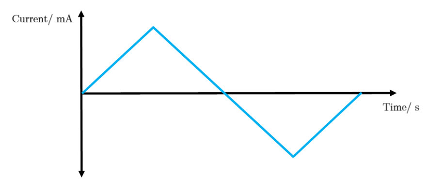
Instead of having to manually plot IV characteristics, as done in 3.3.1, the software can be configured to do this in seconds. An IV characteristic must be drawn when any new sample is placed onto the probe-stick to ensure the chosen current obeys Ohm’s law. Firstly, the software parameters are altered such that 50 measurements are taken per single period; where the period is triangular. The reason a triangle period is used, is to correct any thermal EMF caused by the current source. If the current calculated in part 3.3.1 is entered for a sample and the program produces a straight line IV characteristic, the current that was entered is perfect to be used for the experiment. Figure 7 shows the triangle shape:

Figure 7: Image showing the use of a triaangular period to eliminate thermal EMF

3.4.2 - RT calculations

Having achieved a suitable current, the program must be reconfigured to take resistance and temperature measurements to produce an resistance vs temperature graph. Instead of a triangle shaped period, a square shape is used for 4 periods, with 8 measurements per period. The axis are then altered, such that the resistance is on the y-axis and the temperature is on the x-axis.

3.5 - Rotation of pin configuration

With the software configured, an initial resistance-temperature measurement is taken and recorded. The pin-configuration is then rotated by 90° and the program is run again. Another resistance-temperature measurement is taken and recorded. Doing this corrects any inconsistencies in the sample itself. This step is vital and will be used for analysis, such as in the Van der Pauw equation.

Figure 8: Image showing the rotation of pin configuration by 90 degrees

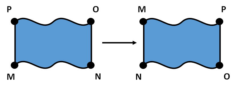
3.6 - The Van der Pauw Equation

The aforementioned Van der Pauw equation is a way of calculating the resistivity whilst also eliminating any potential geometrical inconsistencies in the sample. Once a resistance measurement is recorded, another is also recorded after the rotation of the 4-pin configuration by 90°, as shown in figure 8. The resistance of the samples is calculated from the 4 pins sysetematically; a current is driven between two contacts, the voltage is then measured between these two contacts and the resistance is found simply by using Ohm’s law, V=IR. The equations used to calculate the resistances are:

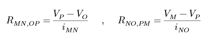
To calculate the resistivity, ρ, of a sample with a thickness, d, this equation must be solved numerically:

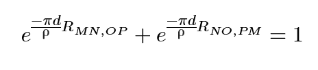
Solving this equation gives the Van der Pauw equation which can now be used to calculate the resistivity. The equation is as follows:

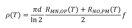
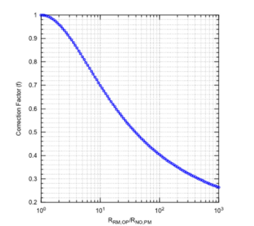
The correction factor, f, is a universal value that is obtained from a graph, shown in figure 9. It depends on the ratio of the two resistances, where the smaller resistance is always divided by the larger one.

Figure 9: The universal graph used to determine the correction factor from the ratio of resistances [1]

The uncertainty in calculating a resistivity using the Van der Pauw equation is:

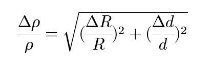
The uncertainty of the resistivity can be simplified to 4% of the calculated value for this particular experiment. This is explained in the appendix.

3.7 - Dipping of the probe-stick

Having calculated an initial resistivity using the Van der Pauw method, the probe-stick can now be dipped into the Helium tank to acquire a reistance-temperature relation. The probe stick, with the sample in place, is locked onto the helium tank, and dipped at a rate of 10Kmin-1. Once the temperature of the melting point of Helium is reached (4.2K), the software is stopped and the newly plotted graph can be analysed. The probe stick is taken out at the same rate it was lowered into the Helium tank and is left to cool for the next sample. The data is analysed on Origin.

If you have any questions, leave them below and until next time, take care.

~ Mystifact

---

References:
[1]: Ramadan, A, et al. 1994. On the vdP method of resistivity measurements. Thin Solid Films. 239. 272-275

Please note; no copyright infringement is intended. All images used have been labelled for re-use on Google Images. If any artist or designer has any issues with any of the content used in this article, please don’t hesitate to contact me to correct the issue.

Previous LET chapters:
Chapter 1 - Abstract
Chapter 2 - Introduction

Next chapter:
Chapter 4 - Results and Discussion

Follow me on: Facebook, Twitter and Instagram, and be sure to subscribe to my website!