UNIFORM CIRCULAR MOTION: POSITION VECTOR, VELOCITY AND ACCELERATION
Hello comunity of steemit, after a time I'm coming back with an article dedicated to the teaching of physics, and in this opportunitid I wanted to wrote about the circular uniform motion. because many books made a short treatment about the vectors position, velocity and acceleration. As a professor of basic physics that I am, when I have to teach this motion I explain this point of the issue to do more complete the knowledge as well as show the utility of vectors in motion.
Say this, let get started...
The uniform circular motion (UCM) is one in which the mobile moves describing a circular path (circumference). This circumference has a radius (which is a characteristic element of it). In this type of movement the displacement is not linear but angular; however, a connection between the linear and angular displacements can be established.
Figure 1 shows a mobile, represented by a car that has moved an angle Δθ = θf - θi measured from the positive x axis and travels an arc length ΔS = Sf - Si, this arc is a curve that represents part of the circumference. Therefore it is a length which is not angular (it is measured in units of length) and all this occurs during a time interval Δt = tf - ti. Also we can see the radius of the circumference which goes from the center of this to any point of the circle. It is important to note that the angular displacement Δθ is uniform, which means that in the given time intervals Δt the same angular displacement is made.
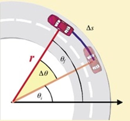
Figure 1: Representation of the Circular Uniform Movement, image taken from: https://www.fisic.ch/contenidos/cinem%C3%A1tica-rotacional/mcu/
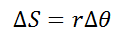
Applying the geometric equation to calculate the arc length, you can find the relationship between radius, angular displacement and arc displacement:
 (1)
(1)
Note that the changing quantities in this equation are the arc length and the position or angular displacement, while the radius remains constant because it complies with its geometric definition.
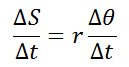
The other element that presents changes is time. Therefore, considering the temporal variation we have:
 (2)
(2)
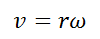
The quantity ΔS / Δt represents the magnitude of the linear velocity v of the mobile in UCM which is constant (in magnitude). The quantity Δθ / Δt represents the measure of the change of angular position with respect to time, this is called angular speed, it is represented by the Greek letter omega (ω), this speed is measured with the units radians per second (rad/s) and since the change in angular position is uniform, then ω is constant, for this reason it is called uniform circular motion. Equation (2) can be rewritten:
 (3)
(3)
Where we can see the relationship between angular displacement and linear displacement. The units of ω in the international system of units is the radian / second (rad / s).
If the limit is taken in equation (2) when Δt tends to zero on the right side of equality we will have:
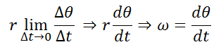 (4)
(4)
Now, expressions for position, velocity and acceleration in uniform circular motion in vector form will be deducted.
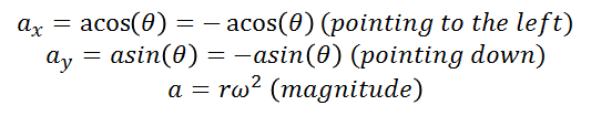
Figure 2.I shows the circular trajectory of the particle represented by the point P. The radius of the circumference is the radio vector that allows locating the particle on the circumference; r will be a vector whose rectangular components are rX and rY. For the angular displacement, we will consider θi = 0 and ti = 0 as initial conditions, in such a way that the angular displacement Δθ = θ and the rotation we will take it in counterclockwise direction.
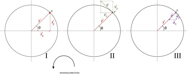
Figure 2: I) Position vector, II) Velocity vector, III) Acteleration vector and their corresponding comopnents for a particle in Uniform Circilar Motion located at the point P. Image edited by the author using Microsoft Powerpoint 2010.
Applying basic trigonometry we have:
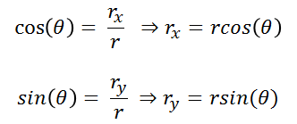 (5)
(5)
Considering r as a vector, this can be written in terms of the rectangular unit vectors i and j as follows:
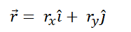 (6)
(6)
Substituting equation (5) in (6):
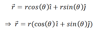 (7)
(7)
From this equation we can see:
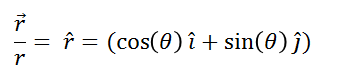 (8)
(8)
This last expression shows us the radial direction (unitary vector r) of the vector position.
As can be seen, the magnitude of the position vector is precisely the value or measure of the radius of the circumference and the signs of the components in terms of i and j denote what we observed in Figure 2.I, the vertical component points upward (positive y) and the horizontal component points to the right (positive x).
The velocity vector is obtained by computing the derivative of the vector position with respect to time:
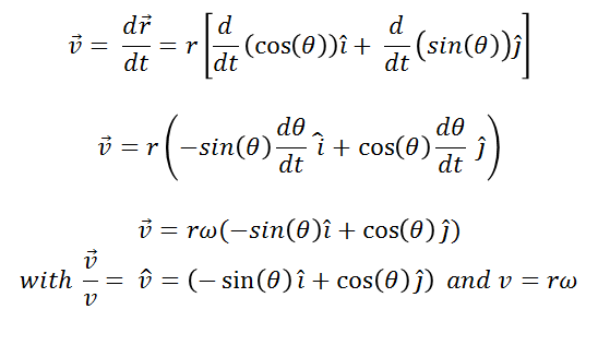 (9)
(9)
The equations (9) give the rectangular components vX and vY of the velocity and tells us that the horizontal component points to the left (negative x) and the vertical component points upwards (positive y). Furthermore, it is also obtained from equations (9) that the magnitude of the velocity is rω as obtained in equation (3).
Figure 2.II shows the components of the velocity vector. By summing these components vectorially, we graphically see the velocity vector and observe that it is tangent to the circumference. Another result of equations (9) shows that the magnitude of the velocity is constant, but the direction does vary. Therefore, since the magnitude of the velocity vector is constant, there is no tangential acceleration. Likewise, Figure 2.II reveals that the velocity vector is perpendicular (or normal) to the position vector r.
Taking the derivative of the velocity with respect to time (that is, equation (9) is derived with respect to time), we will obtain the acceleration of the mobile that describes a circular trajectory:
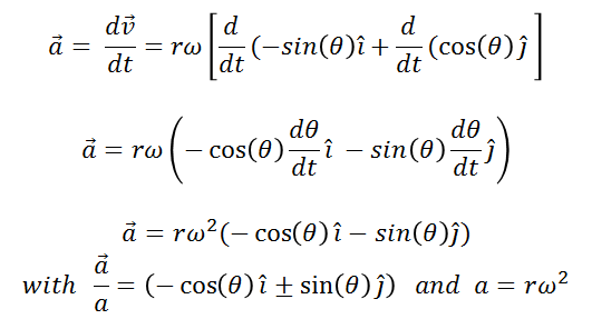 (10)
(10)
Equation (10) says that the horizontal component of the acceleration vector points to the left (negative x) and the vertical component points down (negative y) and when we do the vector sum, we see that the acceleration has the same direction of the position vector r (radial direction) and points towards the center of the circumference, this is known as "centripetal acceleration" (which means directed towards the center) as shown in figure 2.III.
These results have been deduced by applying basic mathematics, but what does physics say? In figure 3 we see some examples. Figure 3.I shows a person spinning an object (a stone or a ball) that is tied to a string which will provide the radius of the circular path. The tension in the rope will produce a "pull" towards the hand that holds it (where the center of the circumference is). This confirms the presence of centripetal acceleration. On the other hand, if the string breaks, the object will shoot straight and tangent to the circumference, showing that the linear velocity is tangential.
Figure 3.II shows a gear or sprocket that fits into a straight (or linear) gear. When the gear rotates, it transmits its rotational movement to the other piece, which will move in a straight line tangent to the gear, this corroborates the relationship between linear and circular motion.
Figure 3.III shows the moon spinning in a uniform circular orbit around the earth. The "invisible" rope that ties the moon to the earth is gravity, which from the center of the moon to the center of the earth (geometric center of the circumference described in the orbit).
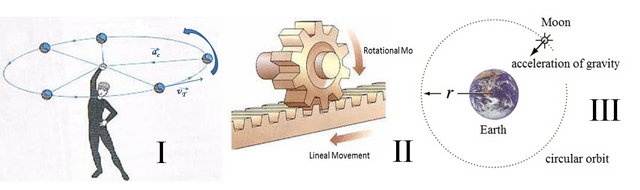
Figure 3: I) relationship between centripetal acceleration, tangential velocity and the circular path, II) relationship between angukar motion and lineal motion, III)example of CUM on the orbot of thr Monn around the Earth. Images taken from:
https://colcafe.wordpress.com/movimiento-circular-uniforme/
http://www.profesorenlinea.cl/fisica/MovimientoCircular.html and
http://hyperphysics.phy-astr.gsu.edu/hbasees/orbv.html
and esdited by the author using Mirosoft PowerPint 2010.
The components of velocity vector and acceleration vector were obtained by applying derivatives, but they can also be obtained by applying geometry in the following way. With reference to figure 2.II, extracting from it the velocity vector, its components and showing the angular relation with the angular displacement θ, this is observed in figure 4.
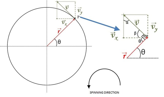
Figure 4: Diagram to show th rectangulars components of the velocity vector, and some angulars relations to obtain the vector velocity using geometry. Image edited by author using Microsoft PowerPoint 2010.
In the figure we see that the angle θ is repeated in the angle between the vector r and the x component of the velocity, in addition it is also deduced that between the velocity vector and the position vector there is 90 °. From there you have:
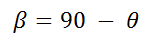 (11)
(11)
On the other hand, if the theorem of the sum of the internal angles of a triangle is applied:
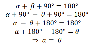 (12)
(12)
When applying trigonometry based on the angle θ we finally find the components of the velocity vector:
 (13)
(13)
In the case of acceleration, the geometry based on the angle θ and its relation to the components of the acceleration vector is easier to see. With reference to figure 2.III, figure 5 is extracted.
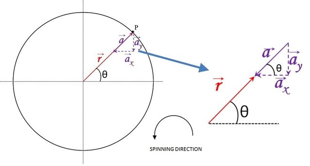
Figure 5: Diagram to show th rectangulars components of the acceleration vector, and some angulars relations to obtain the vector acceleration using geometry. Image edited by author using Microsoft PowerPoint 2010.
It can be noted that θ between the vector r and the x axis is repeated in the angle formed between the vector a and its horizontal component because they are corresponding angles.
Applying trigonometry, we find the horizontal and vertical components of the acceleration vector:
 (14)
(14)
As can be seen, the results of the components of the velocity and acceleration vectors were obtained in the first quadrant (see figure 2, there is shown the circle divided into 4 parts or quadrants), if these same results are applied in the second quadrant, the result shown in figure 6 is obtained.
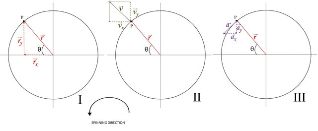
Figure 6: Diagram showing a "wrong" plott of the components of the vectors position, velocity and acceleration in the 2nd quadrant, the mistake is in the position of the angle θ. Image edited by author using Microsoft PowerPoint 2010.
We see in the figure that the results do not agree with what we have already proven. But if we observe well, θ is not in the right place (see figure 6.I), θ should be taken starting from + x and in this case the initial conditions have been considered θi = 0 in you = 0. Therefore if θ is an angle that is in the second quadrant starting from + x and counterclockwise, θ> 90 °. In this case:
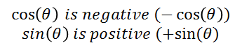 (conditions for the signs for si and cosine for angles located in the cecond quadrant)
Thus, the components of the position, velocity and acceleration vectors are written as follows:
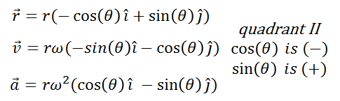 (15)
(15)
Applying the same reasoning in the third and fourth quadrants, we have the correction to the position, velocity and acceleration vectors, the results are shown in figures 7, 8 and 9.

Figure 7: Diagram showing the correct plott for the vector position, velocity and acceleration in the 2nd quadrant. Image edited by author using Microsoft PowerPoint 2010.
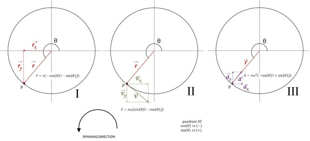
Figure 8: Diagram showing the correct plott for the vector position, velocity and acceleration in the 3rd quadrant. Image edited by author using Microsoft PowerPoint 2010.
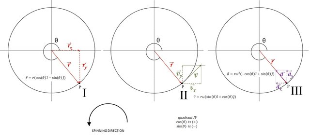
Figure 9: Diagram showing the correct plott for the vector position, velocity and acceleration in the 4th quadrant. Image edited by author using Microsoft PowerPoint 2010.
We can write the magnitude of the centripetal acceleration in terms of the magnitude of the tangential velocity and the radius of the circumference described as follows:
 (16)
(16)
Some books or articles relative to this issue use to write the angular displacement θ in terms of the angular speed ω and time t because:
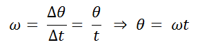 (17)
(17)
So we only have to change the value of θ in all equations where it appears. We are considring again the initial conditions: θi = 0 and ti = 0 in equation (17)
Finaly, when the particle has completed a cycle, the entire angular displacement is 2π radians, and the time to reach this is known as period and is represented by T, wich is measured in seconds (in units of the International System of units). Likewise, we can count the number of turns made for a mobile in UCM per seconds, this is called frquency, and its units are 1/second or Hertz. However, in practice is more used the frequency i terms of numbers of turns per minute or revolutions per minute (rpm). The period and the frequency are related because they are reciprocal, in other words, T = 1/f or f = 1/T
So if we use the relationship between the angular speed, angular desplacement and time we will have:
 (18)
(18)
I hope this article help You to understand better this kind of motion wich is classified as a motion in two dimentions, in this work I have made an exposition of a part of this issue that some books of basic physics does not explain, especially the geometric part.
If You like this article I would appreciate Your support, and if the article reach enough votes I will write a second part explaining the vector relationship between the angular and linear velocities.
Thanks for view and if You have any questions or constructive criticism I will glad to interact with You in order to improve this article.
References:
Sears and Zemansky vol 1: Universitary Physics 12 ed, 2009, Addison - wesley
https://www.quora.com/What-is-the-direction-of-acceleration-of-particle-in-a-uniform-circular-motion
https://www.fisic.ch/contenidos/cinem%C3%A1tica-rotacional/mcu/
https://colcafe.wordpress.com/movimiento-circular-uniforme/
http://www.profesorenlinea.cl/fisica/MovimientoCircular.html