A comparative analysis of methods mimetics, finite difference and finite elements for stationary problems

Greetings to all! Welcome to my Blog. I would like to share in this opportunity with all of you dear readers, a very important topic in the area of mathematics and numerical analysis, as is the comparison of some classical numerical methods with a novel method, but of great importance in recent decades; the classical methods are the method of finite differences and the method of finite elements, and the novel method is the method of mimetic finite differences or commonly known in literature as the mimetic method, such comparison or analysis will be from a numerical point of view. This comparison seeks to conclude about the efficiency, and the order of convergence of these methods. For them we will base ourselves on studying the performance of these methods with one-dimensional border value problems (BVP) (convection-diffusion equation in stationary regime) with different variations in gradient, diffusive coefficient and convective velocity. This publication is the product of a research project in the area of Computer Science. It is aimed at an audience with experience in numerical analysis. I hope it is to your liking, and the results that we will show below will be very useful. Without wasting any more time, let's get started.

---

---

The finite difference method and the finite element method are the most used numerical methods to obtain solutions of problems that appear in many applications, which are modeled by partial differential equations. In the past few years a growing interest has been focused on conservative finite difference schemes, originally known as operators support and then as mimetic methods [4, 9, 10, 13]. In [6, 7] were shown that the mimetic method exhibits a better performance than the finite difference method.

The finite difference method and the finite element method exhibit advantages and disadvantages depending of the problems that we are facing up. Despite of the drawbacks of the finite element method the last one still prevail in applications nowadays, and in those applications where the finite difference method is much suitable, the standard finite element method has been modified in order to optimize the performance. For instance in problems of fluid dynamics we refer the reader to [11, 12], in problems with discontinuous conductivity see [5]. In [1, 8], the authors compare the efficiency of the mimetic method with finite difference method, basically applying the methods to elliptic problems. To our knowledge the comparison between the finite element method and the mimetic one, so far has not been studied. The experts coincide that this is a hard problem due to the high complexity that arise from the point of view of computational implementation.

The main goal of this work is to compare the finite element method with mimetic one. More concretely, we focus our attention to: convergence, tune up the precisions on the boundary conditions, flexibility in the implementation and computational cost. All the analysis is performed around of the convection diffusion equations for one dimensional stationary problems. In this studied we are going to involve the known results about the comparison between the mimetic method and the finite difference method, in order to get a global chart of the finite difference method and finite element method versus the mimetic one.

---

---

Let us consider the following equation

subject to the boundary conditions


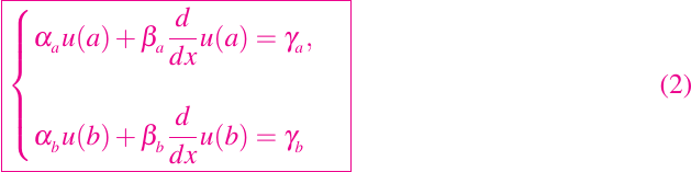
Basically the equation (1) describe the heat propagation via convection–diffusion in stationary regime. The function u(x) represents the temperature at a point x in Ω, k > 0 is the coefficient of thermic diffusion, ν is the convection or advection speed and f is scalar function that describes the existence of a source or sink for the problem. The real parameters {α_i, β_i, γ_i }, i = a, b, take different values depending of the boundary conditions, i.e. Dirichlet, Neumann or Robin boundary conditions.

It is worthwhile to point out that the solution to the equation (1) subject to the boundary conditions (2) can be obtained explicitly by analytical methods. Actually we will strongly use this fact in order to establish the comparison chart between the three already mentioned numerical methods.

---

---

In this section we briefly describe the three methods that we will use along this investigation. The readers interested in more detail about the mimetic method we refer to [9], about finite element method see [3, 15] and the finite different method see [14].

The mimetic methods are based on the discretization of the classical operators: divergence, gradient and curl, assuming that the discretization must satisfy a discrete version of generalized Gauss’s theorem, i.e. the following identity must holds

Where, D, G and B are the discretizations of gradients (∇), divergences (∇·) and ∂/∂n, respectively. By using the identity (3) we obtaine the following relationship between the operators D, G and B


Let us define


where A = Q, or P or I, which are matrices obtained along de process of discretization.

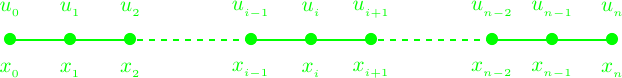
Let us consider a mesh with is given by the nodes x_i , with i = 0, 1, . . . , N, and cells [x_i-1, x_i], for i = 1, . . . , N. Assuming that the mesh is uniformly distributed, h = 1/N. The intermediate point of the cell is given by x_i+1/2 = (x_i + x_i+1)/2. The solution of the problem (1)–(2) and the value of divergence are computed in the middle point of each cell, and the value of the gradient is calculated in the nodes; i.e. in x_i. See figure attached.

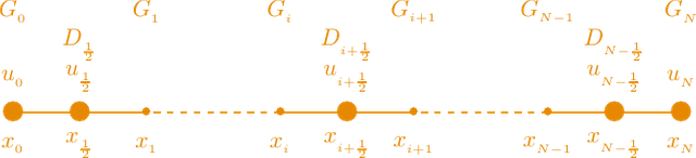
_{One dimensional mesh for the mimetic method.}

The mimetic method arising from a second order discrete operators introduced in [4] is given by formulae (5) and (6).

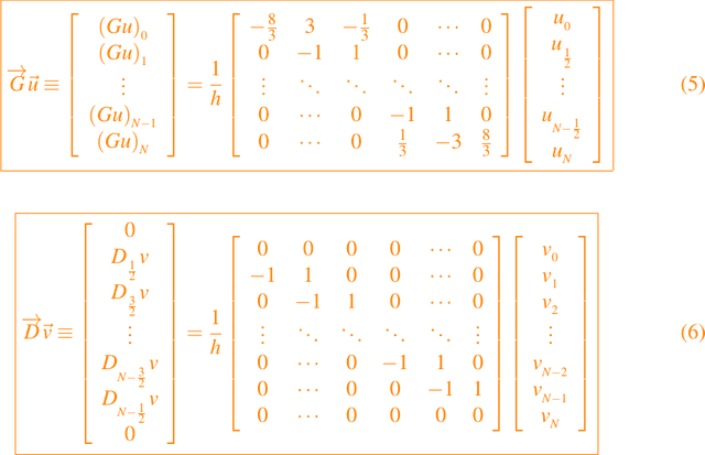
In (6) we add two rows identically equal zero. This is done for technical reason in order that de product between matrices be well defined.

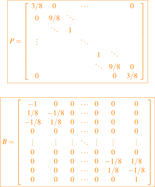
The operator P and B are given by

The discrete versions of the problem (1)–(2) by using the mimetic approach is given by

where U denote the so-called the mimetic solution to equation (7); i.e.


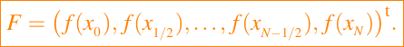
and F is given by

Take into account that the divergence does not play any role on the boundary conditions, we obtain that the Robin boundary conditions is given by

where the vector f_b = (γ_a, 0, . . . , 0, γ_b)^t. Matrices [α] and [β] are such that

α_1,1 = α_a, α_{N+2,N +2} = α_b, β_1,1 = β_a, β_{N +2,N +2} = β_b

and the other entries are equal zero.

Finally, from (7) and (8) we obtain the mimetic scheme for our problem which is given by

Basically, the finite differences method consist in the discretization of the differential operators involved in the problem, assuming that the mesh consist in N + 1 nodes, namely x_i, see figure attached

_{One dimensional mesh for the finite difference method.}

We obtain the following formulae for the first an second derivatives of the solution of the problem

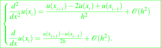
Now, restricting our attention to the equation (1) with Robin boundary conditions (2) the finite difference method give us the following scheme for the computation of the numerical solution of the problem (1)–(2)

where A_i = k_i − ν_i(h/2), B_i = k_i + ν_i(h/2), for i = 1, . . . , N + 1.

Let us assuming, that we already have defined a concrete problem. The finite element method consists in looking for the solution of that problem in the form

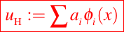
where the coefficients ai are unknown and have to be determined along of an iterative process. The functions φ_i are a base for a finite–dimensional space V_H ⊂ V , and V is a suitable space where we are going to solve the weak or variational form of the following problem, in our case we choose V the Sobolev space H¹(Ω)


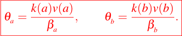
where the bilinear form B(u, v) and the linear functional l(v) are given by, respectively


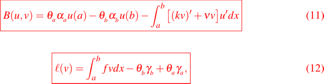
where θ_a and θ_b are given by

---

---

Let us remind that we are dealing with the problem (1)–(2) on the domain Ω = (0, 1). Along this work we are going to estimate the error in computations by using the following norms

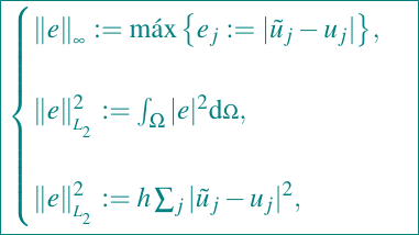
i.e., the norms of the spaces L_∞ and L₂ the continuous and discrete version (see [2]). ũ_j denotes the numerical solution obtained by each of the above mentioned numerical methods and u_j denotes the exact solution of the problem (1)–(2). For the finite difference methods and finite element methods j = 1, . . . , n - 1. For the mimetic methods j = i + 1/2, with i = 0, · · · , n - 1.

Let us solve the problem (1)–(2) with diffusion coefficient k = 1, convective velocity ν = 0, Robin boundary conditions

where


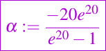
and the source term f(x) is defined in such a way that the exact solution (the black curve in the graphics) is given by


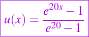
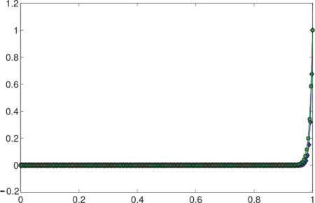
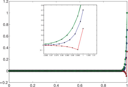
In the following figure, we exhibit the graphic of the exact solution versus the numerical solutions obtained by using the three numerical methods mentioned. The grid is chosen uniformly distributed formed by 20 nodes.


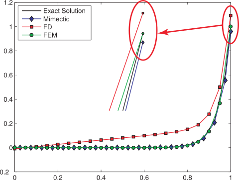
_{Comparison of the approximate solutions on a 20 mesh nodes. At the border, the FEM precision than in the
other two schemes.}

Let us point out that in x = 1, i.e. in the right border, the finite difference methods loose accuracy, even by using second order scheme in order to approximate the boundary conditions. This pathology remains even increasing the number of nodes of the grid and changing the coefficients values k and ν. The three methods give us is suitable approximation when the problem (1) is subject to Dirichlet boundary conditions. The described situation is depicted in the zoom up (see the red oval in figure) of the behavior of the numerical solutions closed to the boundary x = 1.

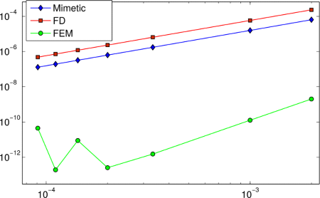
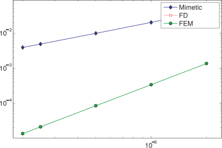
In the following figure we sketch the magnitude of the errors performed by the three methods that we are using along this work. In the left graphic the error is measure by using the norm of L_∞ and in the right one, we use the norm of L₂. In both graphics below the slopes of the straight line mean the convergence order of each numerical method; the best resolve is achieved minimizing the value of the slopes.

Numerical errors the norm L∞.	Numerical errors the norm L2.

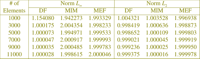
In the chart folowing, we show the theoretical order of convergence of the numerical methods in the norm of L_∞ and in the norm of L₂ .

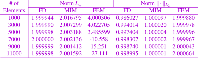
_{Order of convergence in norm L∞ and norm L2.}

However, the maximum norm for this problem, the finite element method has a superconvergence reaching ε machine. Therefore, the oscillations having the graph to the case of finite element method is due to rounding errors rather than machine precision loss finite element method. This feature is not held in other configurations of the problem as will be seen later. The norm L₂, the finite element method has a second order in their convergence (as expected, see [15]), while the other two methods have a first order convergence (see figure and chart previous).

Once again, let us consider the problem (1)–(2), where the diffusion coefficient is given by

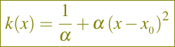
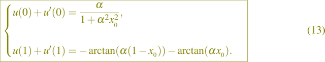
the convective velocity is ν(x) = k'(x), with α = 250 and x₀ = 0.75, and the Robin boundary conditions are given by


The function f(x) is determined in such a way that the analytical solution of our problem is

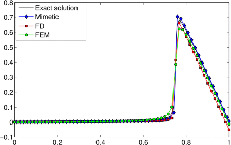
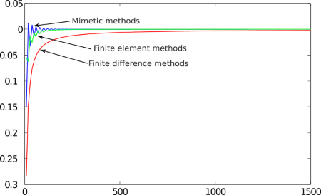
In the following graphic on the left we compare the exact solution versus the approximating one by using a uniform grid formed by 60 nodes. In the other graphic two de right hand side, we ilustrate the asymptotic convergence of the approximating solutions closed to x = 1, as h → 0.

Approximate and exact solutions in a grid of 60 nodes.	Convergence of the methods in the edge node x = 1 as the number of nodes is increased in the mesh.

Let us point out that when the grid is formed just by a few nodes the approximating solutions obtained by mimetic methods exhibits a little bit accuracy over the approximating solutions obtained by the finite element method. In order that the finite difference method can exhibit a better performance in comparison with the two other methods, the grid has to be formed by at least 1500 nodes. If in (13) we set u(0) = u(1) = 0, the best approximating solutions of our problem is obtained by the finite element method.

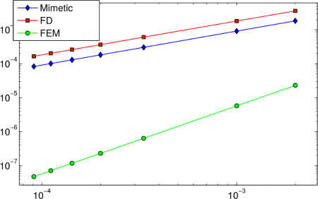
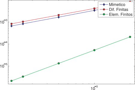
In the figure and following chart we depict the comparison of the error and convergence order performed by the three methods that we are using along this research. Let us remarks that by using the norm of L_∞ to measure the error and the convergence order the finite difference method decrease the order of convergence. This fact is due to that the diffusion and convective coefficients depend of the spatial variable. Despite of this the mimetic methods and finite element method preserve the order of convergence. By using the norm of L₂ and performing the same analysis carried out above, we basically obtained the same results.

Numerical errors the norm L∞.	Numerical errors the norm L2.

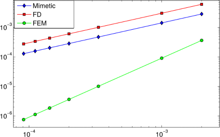_{Order of convergence in norm L∞ and norm L2.}

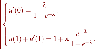
In this section, we are going to consider the problem (1)–(2), setting k = 1.052, ν = −110.5 and f ≡ 0. In this configuration the exact analytical solution is given by

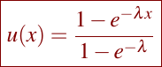
with λ = ν/k. In the numerical implementation we choose the Dirichlet boundary condition u(0) = 0 and u(1) = 1 and in the second experiment the boundary conditions are of the Robin’s type, i.e.

For the problem (1)–(2) with Dirichlet boundary conditions, it is well known that finite difference and finite element methods give us more or less the same result; exhibiting both methods oscillations if the Peclet’s number satisfy that

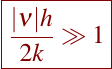
In other words the numerical methods are producing spurious solutions. In order to overcome this drawbacks is by taken h small enough or by adding artificially a diffusion coefficient. It is worthwhile to point out that when the Peclet’s number is less or equal one both methods do not exhibit this pathology on the contrary that Batista and Castillo asserted in [2].

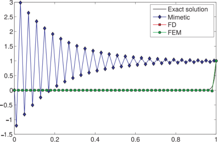
In the following figures we depict the solutions obtained by using a uniform grid with 50, 80 and 200 nodes, respectively. From the numerical experiments turn out that the appearence of oscillations depends of the number of nodes of the grid, by increasing the number of nodes the mimetic methods give us a suitable approximating solution wich uniformly convergences to the exact solution.

Approximate and exact solutions to 50 elements.	Approximate and exact solutions to 80 elements.

Approximate and exact solutions to 200 elements.

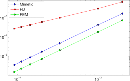
In the figure and following chart it is shown the errors and the order of convergence performed by the three involved numerical methods subject to Dirichlet boundary conditions. By using the norm of L_∞ the finite difference and finite element methods exhibit more or less the same behavior and maintain the convergence order two. However the mimetic method loses the convergence order two and in comparison with the two other methods his performance is much weak. By usin the norm L₂ the finite difference method and the mimetic method show an order of convergence one. The finite element method in the norm L₂ preserves the convergence order two and ones again his performance is much robust. Comparing these results with those one obtained in the example 2, it is quite clear that the same advantages and drawbacks of the methods prevails.

Numerical errors the norm L∞.	Numerical errors the norm L2.

_{Order of convergence in norm L∞ and norm L2.}

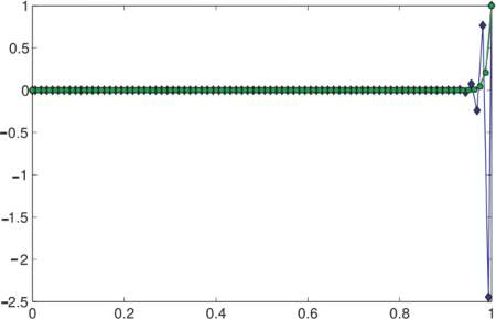
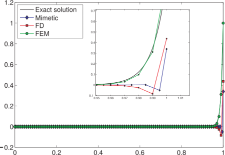
Let us consider the problem (1)–(2) subject to the Robin’s boundary conditions. The result of the numerical implementation of this problem is exhibit in figure following. In x = 1 the finite difference method and mimetic method exhibit a very poor performance, as it is shown in the zoom up of the graphics. The mimetic method in some cases needs even 4000 nodes in order to reach the precision of the finite element method wich just need 80 nodes in the grid. The finite difference method loose the precision at x = 1, and the method diverges.

Approximate and exact solution 100 elements. The extended part of each graph represents the numerical behavior around the border x = 1.	Approximate and exact solution 200 elements. The extended part of each graph represents the numerical behavior around the border x = 1.

---

---

First of all we point out that finite element method exhibits a better precision in obtaining the numerical solution as well with the convergence order than the other two methods. Moreover the mimetic method exhibits a better performance than finite difference method. This fact has been mentioned by difference researchs [1, 7, 8]. In the example three the mimetic method can not reach a better performance than the others method, on the contrary that we would expected due to the conservative character of the mimetic method.

From the research it follows that much work has to be done in this direction. The mimetic and the finite difference methods prevail over the finite element method for problems in one dimensional spaces. Basically this fact is due to that the mimetic and finite difference methods are much easiest their numerical implementation. However in higher dimensions, even in two dimensional spaces, the three methods present a great difficulties in the discretization process. Moreover if we want to increase the convergences order arise a lot new difficulties.

---

---

1. J. Arteaga and J.M. Guevara. A conservative finite difference scheme for static diffusion equation. Divulgaciones Matemáticas, 16(1):39–54, 2008.
2. E.D. Batista and J.E. Castillo. Mimetic schemes on non-uniform structured meshes. Electronic Transactions on Numerical Analysis, 34(1):152–162, 2009.
3. Eric B. Becker, Graham F. Carey, and J. Tinsley Oden. Finite Elements: An Introduction. Prentice-Hall, Inc., New Jersey 07632, 1981.
4. J.E. Castillo and R. D. Grone. A matrix analysis approach to higher-order approximations for divergence and gradients satisfying a global conservation law. SIAM J. Matrix Anal. Appl., 25(1):128–142, 2003.
5. F. Cordero and P. Dı́ez. XFEM+: una modificación de XFEM para mejorar la precisión de los flujos locales en problemas de difusión con conductividades muy distintas. Revista Internacional Métodos Numéricos para Cálculo y Diseño en Ingenierı́a, 26(2):121–133, 2010.
6. M.A. Freites. Un estudio comparativo de los métodos miméticos para la ecuación estacionaria de difusión. Tesis de grado, Facultad de Ciencias, UCV, 2004.
7. Juan M. Guevara, M. Freites, and J.E. Castillo. A new second order finite difference conservative scheme. Divulgaciones Matemáticas, 13(1):107–122, 2005.
8. Juan M. Guevara. Sobre los esquemas miméticos de diferencias finitas para la ecuación estática de difusión. Trabajo de ascenso, Facultad de Ciencias, UCV, Caracas, Venezuela, 2005.
9. James M. Hyman and Mikhail Shashkov. The approximation of boundary conditions for mimetic finite difference methods. Computers Math. Applic., 36(5):79–99, 1998.
10. James M. Hyman, Mikhail Shashkov, and S. Steinberg. Mimetic finite difference methods for diffusion equations. Computers Math. Applic., 6(3-4):333–352, 2002.
11. Ben Q. Li. Discontinuous Finite Elements in Fluid Dynamics and Heat Transfer. Springer-Verlag, London, fifth edition, 2006.
12. Béatrice Rivière. Discontinuous Galerkin Methods for Solving Elliptic and Parabolic Equations: Theory and Implementation. SIAM, Philadelphia, fifth edition, 2008.
13. Mikhail Shashkov and Stanly Steinberg. Support-operator finite-difference algorithms for general elliptic problems. Journal of Computational Physics, 118(1):131–151, 1995.
14. John C. Strikwerda. Finite Difference Schemes and Partial Differential Equations. SIAM, Ltd., Philadelphia, second edition, 2004.
15. Pavel Šolı́n. Partial Differential Equations and Finite Element Method. John Wiley & Sons, Ltd., New Jersey, fifth edition, 2006.
16. Giovanni Calderón y Abdul Lugo, Estimación del error y adaptatividad en esquemas miméticos para problemas de contorno, Boletin de la Asociación Matemática Venezolana, 22(2):109–124. 2015.
17. Abdul Lugo, Generación de mallas óptimas basadas en equemas de discretización mimética para problemas de contorno, Tesis de Doctorado, Facultad de Ciencias, Universidad de Los Andes, Venezuela.
18. Abdul Lugo, Adaptatividad de soluciones usando esquemas miméticos en mallas adaptadas en movimiento. Preprint. 2017.

---

---

The separators and equations were created and edited by @abdulmath using free software, GNU Octave, , GIMP and Inkscape.

---