Bayesian Networks and Their Value - An Essay, Part 1
In the past few decades, Bayesian networks (BNs) have become extremely popular due to the wide variety of problems it can tackle. In short, BNs are graphical models for capturing probabilistic relations between evidence and hypotheses. They have been used for applications in several fields, including forensic, genetics, engineering, risk assessment, machine learning, text mining, natural language processing, speech recognition, medical diagnosis, weather forecasting, and even wine classification (T. Pilditch & Dewitt, 2018). In this paper, I will touch on the role of BNs in medical decision making under uncertainty. The structure found in BNs makes them intuitively appealing while also being convenient for the representation of causal and probabilistic relations. BNs are mathematically rigorous, intuitive, and complex structures. BNs are a mix of prior knowledge and observed data that enable us to gain a deeper understanding of various problem domains. BNs can aid us in predicting the future and understanding our present. For the purpose of this paper, I will describe what BNs are and discuss their practical applications. In addition, I will mention the strengths and weaknesses of BNs as well as their growth potential and future use.
Probabilistic graphical models (GMs) are graphic structures that allow knowledge representation of an uncertain domain. They are tools for handling uncertainty that draw from causal knowledge. In a GM, each node represents a random variable, while each edge between nodes represents a probabilistic dependence between the nodes it touches. The conditional dependencies in the graph are usually calculated by using statistical and computational models. BNs belong to the family of GMs. Therefore, BNs combine graph theory, probability theory, computer science, and statistics. More specifically, BNs belong to a group of GMs called directed acyclic graphs (DAGs). DAGs are particularly popular in the fields of statistics, machine learning, and artificial intelligence. Part of the appeal in BNs is that they enable an effective representation and computation of the joint probability distribution (JPD) over a set of random variables (Pearl, 1988).

Pixabay image source. A spiderweb as a network.
The structure of a DAG is divided into two, the set of nodes and the set of directed edges. Each node is drawn as a circle and represents a random variable. The edges are drawn as an arrow between the nodes, and they represent a direct dependence between the variables. Therefore an arrow from node X to node Y represents a statistical dependence between the variables. In other words, the value taken by node Y depends on the value taken by node X, X influences Y. In that case, node X is referred to as the parent, and node Y is referred to as the child. These connections among variables form chains. When a child node has two or more parents, it is referred to as a “common effect” for those parents. On the other hand, when a parent node has several children, it is referred to as a “common cause” for those child nodes. Finally, the acyclic property of a DAG guarantees that no node can be its own ancestor or its own descendant. Hence, each variable is independent of its non-descendents given the state of its parents. Thanks to this property, the amount of parameters needed to characterize the JDP of the variables is often reduced (Friedman, Geiger, & Goldszmidt, 1997; Pearl, 1988; Spirtes, Glymour, & Schienes, 1993). This reduction enables the efficient computation of posterior probabilities given evidence.
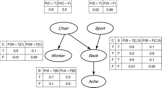
Figure 1. The backache BN example (Ben-Gal, 2008).
The conditional probability distribution (CPD) at each node depends only on its parents. If node X has no parents, then its local probability distribution is said to be unconditional, otherwise it is conditional. For discrete random variables, this conditional probability is often displayed in a table as in figure 1. Each table lists the local probability that a child takes on each of the feasible values for each combination of values of its parents. In figure 1, each child can take the value of True (T) or False (F) depending on the values of its parents. Furthermore, as it becomes clear from figure 1, a BN provides a compact factorization of the JPDs. Factorization of the joint distribution of all variables by the chain rule results in 25-1=31 model parameters for five random variables. Nevertheless, if a BN is used, as in figure 1, we can reduce the amount of parameters to 10. This simplification provides great benefits from inference, learning, and computational perspectives. It is important to note that BNs have a misleading name. The use of Bayesian statistics in conjunction with BNs provides a method to avoid overfitting of the data. However, using BNs does not imply the usage of Bayesian statistics. Actually, many practitioners follow frequentist approaches to estimate the parameters of a BN (Ben-Gal, 2008).
The backache BN example (Figure 1) considers a person who suffers from a back injury denoted by “Back”. The injury produces pain, denoted by “Ache”. The injury might be the product of a contact sport activity denoted by “Sport”. Perhaps the back injury is actually the product of new, uncomfortable chairs installed at work, denoted by “Chair”. If the chair is the culprit, then it is reasonable to think another coworker is suffering from a similar backache, denoted by “Worker”. If a variable is represented by a node, it is said that it is being “observed”. The beauty of BNs is that each node not only represents a random variable, it can also represent a hypotheses, belief, or a latent variable. Therefore BNs help reasoning on evidence but also on suppositions. In this example, it is very clear the two types of inference support that BNs allow. The first type is called top-down reasoning. It provides predictive support for node X based on evidence nodes connected to X through its parent nodes. If the person being considered in the backache BN example played rugby during the weekend and got hit on his lower back, then it provides predictive support of a back injury. The second type is bottom-up reasoning (Ben-Gal, 2008). It provides diagnostic support for node X through its children nodes. Experiencing back pain is diagnostic support of having a back injury. Once given training data and prior information, the parameter of the JDP in the BN can be estimated. Expert knowledge or causal information are considered prior information.
Sometimes, not only do the parameters need to be calculated, but the structure of the BN also must be learned. This is known as the BN learning problem. It splits into four main categories. For the first category, the goal of learning is to find the parameters that maximize the likelihood of the training dataset. In the second category, the structure is known, but there is partial observability. In this case, an expected maximization algorithm can be used to find a locally optimal maximum-likelihood estimate of the parameters. In the third case, the goal is to learn the DAG that best represents a given dataset. One approach is to assume that the variables are conditionally independent given a class which has a single common parent node to all the variable nodes. Such approach is called naive BN and it brings surprisingly good results to some practical problems (Ben-Gal, 2008). Finally, the fourth case occurs when there is partial observability and unknown graph structure. Depending on the problem, different algorithms can be used.
Check out Part 2!
References:
- Bartlett, J. G. (1997). Management of Respiratory Tract Infections. Blatimore: Williams & Wilkins.
- Ben-Gal, I. (2008). Bayesian Networks.
- Castle, N. (2017, July 13). Supervised vs. Unsupervised Machine Learning. Retrieved May 1, 2018, from https://www.datascience.com/blog/supervised-and-unsupervised-machine-learning-algorithms
- de Bruijn, N., Lucas, P., Schurink, K., Bonten, M., & Hoepelman, A. (2001). Using Temporal Probabilistic Knowledge for Medical Decision Making. In S. Quaglini, P. Barahona, & S. Andreassen (Eds.), Artificial Intelligence in Medicine (Vol. 2101, pp. 231–234). Berlin, Heidelberg: Springer Berlin Heidelberg. https://doi.org/10.1007/3-540-48229-6_33
- Friedman, N., Geiger, D., & Goldszmidt, M. (1997). Bayesian Network Classifiers, 33.
- Lucas, P. (n.d.). Bayesian Networks in Medicine: a Model-based Approach to Medical Decision Making, 6.
- Lucas, P. J. F., Boot, H., & Taal, B. (1998). A decision-theoretic network approach to treatment management and prognosis. Knowledge-Based Systems, 11(5–6), 321–330. https://doi.org/10.1016/S0950-7051(98)00060-4
- Pearl, J. (1988). Probabilistic Reasoning in Intelligent Systems. San Francisco: Morgan Kaufmann.
- Pilditch, T. D., Hahn, U., & Lagnado, D. A. (under review). Integrating dependent evidence: naive reasoning in the face of complexity.
- Pilditch, T., & Dewitt, S. (2018, February). Knowledge Learning and Inference Lecture - Bayesian Networks Part 2: Application to Problems. University College London.
- Shachter, R. D. (1986). Evaluating Influence Diagrams. Operations Research, 34(6), 871–882. https://doi.org/10.1287/opre.34.6.871
- Spirtes, P., Glymour, C., & Schienes, R. (1993). Causation Prediction and Search. New York: Springer-Verlag.
Best,
Interesting content as always @capatazche Waiting for part 2 :)
To listen to the audio version of this article click on the play image.

Brought to you by @tts. If you find it useful please consider upvoting this reply.
You have been defended with a 50.00% upvote!
I was summoned by @capatazche.
Great post!
Thanks for tasting the eden!
Hi @capatazche!
Your post was upvoted by utopian.io in cooperation with steemstem - supporting knowledge, innovation and technological advancement on the Steem Blockchain.
Contribute to Open Source with utopian.io
Learn how to contribute on our website and join the new open source economy.
Want to chat? Join the Utopian Community on Discord https://discord.gg/h52nFrV
https://mb2-717-dumps.blogspot.com/2020/09/get-valid-huawei-h13-629v20-dumps.html
https://cs0-001-dumps.blogspot.com/2020/09/the-way-to-pass-exam-with-h35-211-exam.html
https://pass4sure-200-150-dcicn.blogspot.com/2020/09/knowledge-most-current-huawei-h31.html
https://www.olaladirectory.com.au/updated-nutanix-ncp-5-10-exam-preparation-material/
https://medium.com/@azytrend/ace-pdf-questions-perfect-idea-for-ace-test-preparation-2aea76b336e9
https://www.olaladirectory.com.au/brilliant-ncse-core-exam-questions-with-pdf-dumps/
https://www.lily.fi/blogit/exambraindumps/latest-ibm-c1000-056-braindumps-for-huge-success/
http://certificationexam.educatorpages.com/