Machine learning (Keras) and Steem #1: User vs bid-bot binary classification
Repository
https://github.com/keras-team/keras
What Will I Learn?
- Collect and preprocess data
- Visualize dataset
- Build neural network model
- Measure model performance
Requirements
- python
- basic concepts of machine learning
Tools:
- python 3
- pandas
- matplotlib
- seaborn
- jupyter notebook
- scikit-learn
- keras + tensorflow (as backend to keras wrapper)
It looks like a lot of libraries, but it's a standard python toolset for data analysis / machine learning.
Difficulty
- Intermediate
Tutorial Contents
- Problem description
- Collecting data
- Visualization of the dataset
- Building model
- Measuring model performance
- Conclusions
Problem description
The purpose of this tutorial is to learn how to build a machine learning model that will be able to distinguish an user from a bid-bot.
Collecting data
A list of bots has been collected from https://steembottracker.com and can be found here. Now we need list of users. Let's choose those users who added a post in the category #utopian-io in July 2018. We will use the following script and database SteemSQL.
SELECT DISTINCT author
FROM Comments (NOLOCK)
WHERE depth = 0 AND
      category = 'utopian-io' AND
      YEAR(created) = 2018 AND
      MONTH(created) = 7
The obtained list is several times bigger than the bot list, but we will not modify it, because this is very common in machine learning. Rarely data is perfect. The list can be found here: users.txt
Now we want to extract statistics for each account from the list. We will use the beem library.
We will use the following attributes:
- number of followers
- number of followings
- followings / followers ratio
- reputation
- number of users that muted given account
- effective STEEM POWER (with delegation)
- own STEEM POWER (without delegation)
- effective STEEM POWER / own STEEM POWER ratio
from beem.account import Account

bid_bots = set(map(str.strip, open('bid_bots.txt', 'r').readlines()))
users = (map(str.strip, open('users.txt', 'r').readlines()))

with open ('data.csv' , 'w') as f:
    f.write(','.join(['name', 'followers', 'followings', 'foll. ratio', 'muters', 'rep', 'eff. sp', 'own sp', 'sp ratio', 'is bot?']) + '\n')
    for name in bid_bots.union(users):
        account = Account(name)
        foll = account.get_follow_count()
        row = (name,
             foll['follower_count'],
             foll['following_count'],
             foll['following_count'] / foll['follower_count'],
             len(account.get_muters()),
             account.get_reputation(),
             account.get_steem_power(),
             account.get_steem_power(onlyOwnSP=True),
             account.get_steem_power() / account.get_steem_power(onlyOwnSP=True),
             1 if name in bid_bots else 0)

        f.write(','.join(map(str, row)) + '\n')
The result file has been saved as data.csv. A sample of the file is shown below. The last column determines whether an account is a bot, and all previous ones are the attributes which we will use to teach our model.
                 name  followers  followings  foll. ratio  muters        rep       eff. sp        own sp     sp ratio  bid-bot?
0             beggars       1144          66     0.057692       4  58.485711    457.254297    457.254297     1.000000         0
1     anthonyadavisii       3477        2295     0.660052      19  59.185663    575.470517   1210.696343     0.475322         0
2           amvanaken       3026         175     0.057832      10  60.324424    491.175030    716.217811     0.685790         0
3       shaikhraz1986        229          11     0.048035       3  46.766451     15.051121     12.462512     1.207712         0
4            harpagon        306          39     0.127451       0  55.577631    389.858866    389.858866     1.000000         0
5               famil        661         274     0.414523       3  58.858699      7.859833    207.836914     0.037817         0
6           swapsteem        197          31     0.157360       0  39.812361     15.441267      0.907584    17.013591         0
7            kr-nahid        773         366     0.473480       6  58.179101    130.890891    130.890891     1.000000         0
8        thefairypark        153           1     0.006536       0  32.825241     15.000498      0.559973    26.787898         0
9             eosbake        115           0     0.000000       0  25.000000      3.002430      3.002430     1.000000         0
10      official-hord        619         139     0.224556       0  59.131711     65.469489     65.469489     1.000000         0
..                ...        ...         ...          ...     ...        ...           ...           ...          ...       ...
Visualization of the dataset
Let us first look at the dataset. We can expect that:
- more people mute the bots
- bots have a higher effective STEEM POWER
- bots have most of the STEEM POWER from delegation
- bots have a lower average reputation (because they do not add posts)
- bots observe fewer users
Let's check if our assumptions are confirmed.
for c in columns:
    print('%s|%.3f|%.3f' % (c, df[df['bid-bot?'] == 0][c].mean(), df[df['bid-bot?'] == 1][c].mean()))
It turns out that the presumptions turn out to be true. We can see great differences in average values here.
| Attribute | User average value | Bid-bot average value |
|---|---|---|
| followers | 1078.974 | 1926.841 |
| followings | 382.238 | 204.068 |
| foll. ratio | 0.389 | 0.170 |
| muters | 3.524 | 12.330 |
| rep | 55.065 | 45.564 |
| eff. sp | 5494.488 | 224684.003 |
| own sp | 2110.639 | 13383.966 |
| sp ratio | 18.165 | 126.915 |
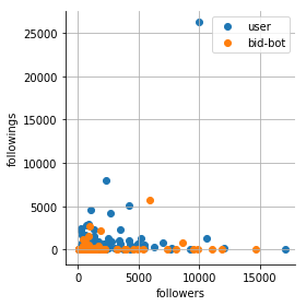
However, calculating the average is not enough. Let's look at some charts.
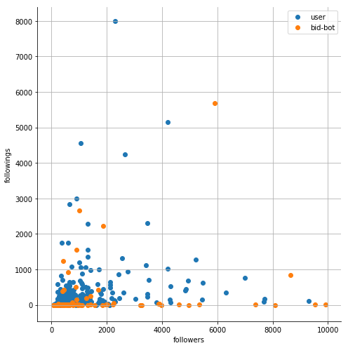
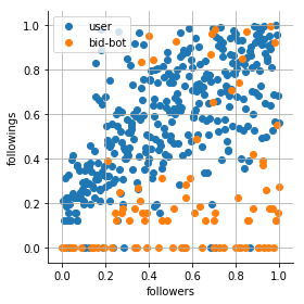
followers + followings:
sns.FacetGrid(df1, hue="bid-bot?", size=7).map(plt.scatter, "followers", "followings")
plt.legend(['user', 'bid-bot'])
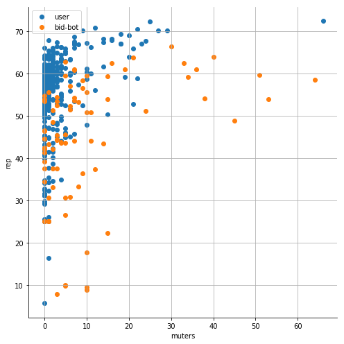
muters + rep:
sns.FacetGrid(df1, hue="bid-bot?", size=7).map(plt.scatter, "muters", "rep")
plt.legend(['user', 'bid-bot'])
foll. ratio + sp ratio:
sns.FacetGrid(df1, hue="bid-bot?", size=7).map(plt.scatter, "foll. ratio", "sp ratio")
plt.legend(['user', 'bid-bot'])
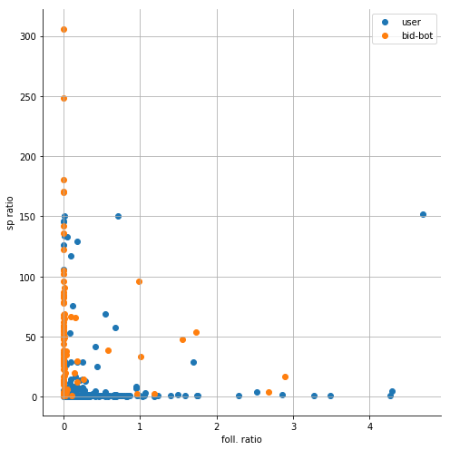
Visualization gives us a much better picture of the situation. We can see that different classes are pretty separable.
Building model
We now have to separate the attributes (X) and the decision class (y), and then split the data into training and test data. The former are used to train the neural network, while the test data are used to check the effectiveness of the classification (it would not be a good idea to teach and test with the same data).
X_cols = ['followers', 'followings', 'foll. ratio', 'muters', 'rep', 'eff. sp', 'own sp', 'sp ratio']
y_cols = ['bid-bot?']
X = df[X_cols].apply(pd.to_numeric)
y = df[y_cols].apply(pd.to_numeric)
X_train, X_test, y_train, y_test = train_test_split(X, y, test_size=0.3, random_state=0)
Our model is a neural network, consisting of:
- the input layer to which the input is transferred
- the hidden layer
- the output layer which returns the classification result
The code building the neural network model is relatively simple.
model = Sequential()
model.add(Dense(24, activation='relu', input_dim=8))
model.add(Dense(12, activation='relu'))
model.add(Dense(1, activation='sigmoid'))

model.compile(loss='binary_crossentropy',
              optimizer='adam',
              metrics=['accuracy'])
model.add - adds new layer
Dense - fully connected layer
relu - ReLU activation function
sigmoid - sigmoid activation function
binary_crossentropy - measures the performance of a classification, where output is a probability between 0 and 1
adam - Adaptive Moment Estimation optimizer, basically RMSProp with momentum
accuracy - percentage of correctly classified inputs
We can display the characteristics of the neural network.
model.summary()
_________________________________________________________________
Layer (type)                 Output Shape              Param #
=================================================================
dense_10 (Dense)             (None, 24)                216
_________________________________________________________________
dense_11 (Dense)             (None, 12)                300
_________________________________________________________________
dense_12 (Dense)             (None, 1)                 13
=================================================================
Total params: 529
Trainable params: 529
Non-trainable params: 0
We can see that we have 3 layers:
- the first has 24 neurons
- the other has 12 neurons
- the third has one neuron
Of course, you can set different values here or even add more layers and check what the results will be.
Now is the time to train the neural network. The epochs parameter means how many iterations will be performed, during which the entire data set is used, and the batch_size parameter determines how many data will be used simultaneously.
model.fit(X_train, y_train,epochs=50, batch_size=1, verbose=1)
Measuring model performance
Let's see a summary of the recent learning iterations.
...
Epoch 45/50
305/305 [==============================] - 0s 2ms/step - loss: 3.0651 - acc: 0.8098
Epoch 46/50
305/305 [==============================] - 0s 1ms/step - loss: 3.0651 - acc: 0.8098
Epoch 47/50
305/305 [==============================] - 0s 1ms/step - loss: 3.0651 - acc: 0.8098
Epoch 48/50
305/305 [==============================] - 0s 1ms/step - loss: 3.0651 - acc: 0.8098
Epoch 49/50
305/305 [==============================] - 0s 2ms/step - loss: 3.0651 - acc: 0.8098
Epoch 50/50
305/305 [==============================] - 0s 1ms/step - loss: 3.0651 - acc: 0.8098
Frankly speaking, it does not look good. The loss value should be as close as possible to 0, while the acc value should be as close as possible to 1.
Let's look at the confusion matrix.
y_pred = model.predict_classes(X_test)
cm = confusion_matrix(y_test, y_pred)
print(cm)
It turns out that the classification process has failed completely. All records (except 1) were classified as user. By the way, we see that the acc metric is not entirely reliable if we are dealing with unbalanced classes.
[[101   1]
 [ 30   0]]
We need to make some modifications so that the network correctly classifies the objects. The choice is very wide:
- add new layers
- change the number of neurons in the layers.
- change the optimizer.
- increase the number of epochs
However, there is not much data, so a simple network should be good enough. Maybe the problem is in the data itself? Let's try to make some preprocessing before adding them to the neural network. As we have seen in the previous charts, the attribute value ranges are quite large. However, for a neural network it is better if these ranges are as close as possible to [0, 1]. That is why we will normalize the input data. We will first try StandardScaler, which standardizes features by removing the mean and scaling to unit variance.
X = pd.DataFrame(StandardScaler().fit_transform(X))
X_train, X_test, y_train, y_test = train_test_split(X, y, test_size=0.3, random_state=0)
model.fit(X_train, y_train,epochs=50, batch_size=1, verbose=1)
y_pred = model.predict_classes(X_test)
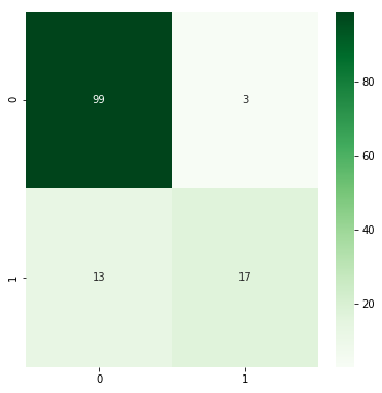
cm = confusion_matrix(y_test, y_pred)
plt.figure(figsize = (4, 4))
sns.heatmap(cm, annot=True, cmap="Greens")
print('precision:', precision_score(y_test, y_pred),
'\nrecall:', recall_score(y_test, y_pred),
'\nf1:', f1_score(y_test, y_pred))
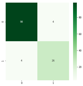
As we can see the results are much better - the loss has decreased, the acc has increased, the confusion matrix looks much better. However, these results are still far from ideal.
Epoch 50/50
305/305 [==============================] - 0s 1ms/step - loss: 0.1310 - acc: 0.9410
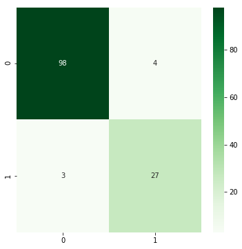
Let us now take a different approach to normalization: QuantileTransformer.
X = pd.DataFrame(StandardScaler().fit_transform(X))
The results are already acceptable.
We were using the number of iterations equal to 50 all the time, let's see what the result will be if we reduce the number of iterations to 10.
model.fit(X_train, y_train,epochs=10, batch_size=1, verbose=1)
It turns out that the result is basically the same and a large number of iterations were not necessary.
Let's look what is the difference between raw data and normalized data.
| Raw data | StandardScaler | QuantileTransformer |
|---|---|---|
 | 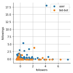 |  |
It turns out that StandardScaler is not at all a very good choice, because the data are not in the range of [0, 1]. And the QuantileTransformer made the data not only in the range of [0,1] but also evenly distributed throughout the area.
Conclusions
- building the optimal model requires experimenting
- it is worthwhile to examine how the input data looks like
- proper preprocessing of the input data is very important
- the decision classes need not be of equal size
- we should try to make the neural network as simple as possible
- not always a large number of iterations is needed
- here we had relatively small dataset, but the bigger the dataset, the better we can train the neural network.
Thank you for your contribution.
Your contribution has been evaluated according to Utopian policies and guidelines, as well as a predefined set of questions pertaining to the category.
To view those questions and the relevant answers related to your post, click here.
Need help? Write a ticket on https://support.utopian.io/.
Chat with us on Discord.
[utopian-moderator]
Congratulations @jacekw.dev! You have completed the following achievement on Steemit and have been rewarded with new badge(s) :
Click on the badge to view your Board of Honor.
If you no longer want to receive notifications, reply to this comment with the word
STOPTo support your work, I also upvoted your post!
Occam's razor principle ;)
All of this topic is at advanced level. I am wondering if eg. SteemPlus uses even similar entry attributes to specify if account is Human or Bot.
You should take any other community than #utopian-io for tests. I believe here are not enough Bot accounts if any.
Very interesting post
Hey @jacekw.dev
Thanks for contributing on Utopian.
We’re already looking forward to your next contribution!
Want to chat? Join us on Discord https://discord.gg/h52nFrV.
Vote for Utopian Witness!