Create Beautiful Charts with Steem Data
What Will I Learn?
Learn to make beautiful charts with Steem block chain data, using free and open source public domain tools.
Requirements
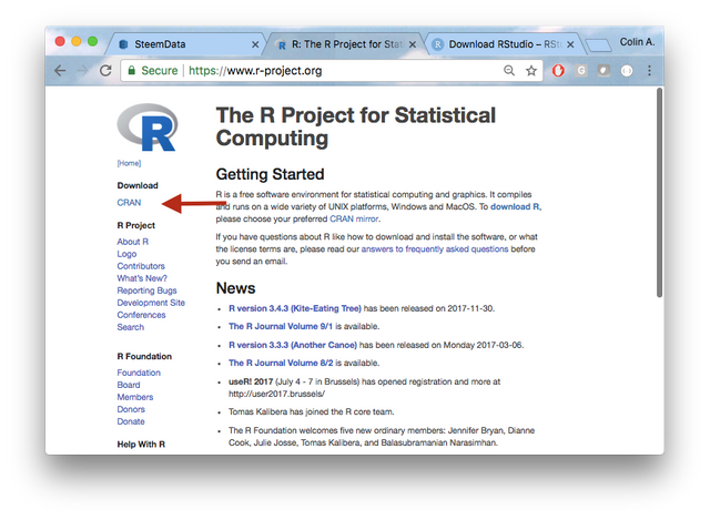
- The free R runtime environment
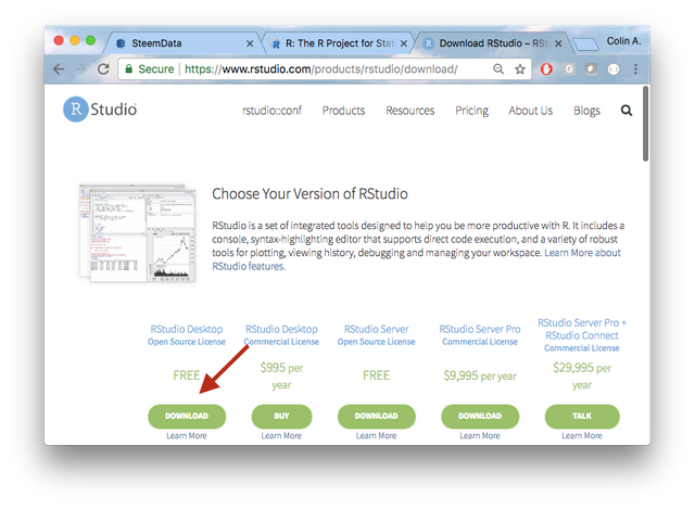
- The free RStudio desktop IDE (Integrated Development Env.)
- Network access to SteemData.com
Difficulty
- Basic
Tutorial Contents
Step 1 - Setting up and loading libraries
Open RStudio and install the libraries we'll be using.
mongoliteis our database driverggplot2is the main graphics packageRColorBrewerwill give us some nice color palettesggthemeshas several nice themes we can work withgridExtrawill allow us an easy way to make panel plots
In the command console type,
install.packages(c("mongolite", "ggplot2", "RColorBrewer",
"ggthemes", "gridExtra"), dependencies = TRUE)
Lets get Data!
Step 2 - Querying steemdata.com
Open a new R Script document and paste in this code and Run the code block. On my Mac the Run shortcut is is CMD+SHIFT+RETURN or from the menus select, CODE >> RUN REGION >> RUN ALL.
   # Load the mongodb database drivers
    library(mongolite)
   # Setup two variables with our date ranges
    sDate <- "2018-01-01T00:00:00.00Z"
    eDate <- "2018-01-31T00:00:00.00Z"
   # Create a database query string
    mdbQuery <- paste('{"timestamp":
                    {"$gte": {"$date": "',sDate,'"},
                    "$lte": {"$date": "',eDate,'"}
                    } }', sep="")
   # Create a conneciton object
    mdb <- mongo(url="mongodb://steemit:[email protected]:27017/SteemData", collection="PriceHistory", db="SteemData")
   # Assign the results of the Query to a new datastructure
    prices <- mdb$find(mdbQuery)
   # Print the first 4 lines of our data structure
    head(prices,4)
After it runs you should see console output like this,
    ##             timestamp  btc_usd  steem_btc    sbd_btc steem_sbd_implied
    ## 1 2018-01-26 15:03:04 10944.32 0.00055113 0.00059930          0.919622
    ## 2 2018-01-26 14:57:59 10947.01 0.00055055 0.00059753          0.921369
    ## 3 2018-01-26 14:52:52 10988.43 0.00055167 0.00059753          0.923239
    ## 4 2018-01-26 14:47:49 11017.92 0.00055175 0.00059759          0.923284
    ##   steem_usd_implied sbd_usd_implied
    ## 1          6.031722        6.558917
    ## 2          6.026868        6.541211
    ## 3          6.061940        6.565952
    ## 4          6.079114        6.584230
Congratulations, we now have Steem bockchain data to work with!
To get a sense of what other data you can access, review this Post.
Lets Plot!
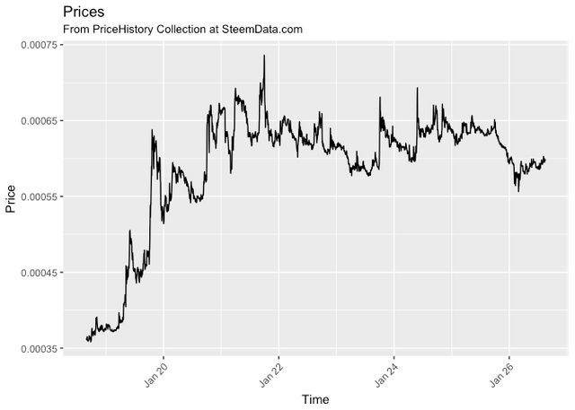
Step 3 - A first plot
Our prices data structure we created in Step 2 is passed into the ggplot function.
If you paste this code into your R Script document and then run it, like you did in Step 2, you should see a base plot.
   # load out base plotting library
    library(ggplot2)
   # Plot the sbd_btc column of our dataset
        ggplot(prices, aes(x=timestamp, y=sbd_btc))+
   # Draw a line plot and interpretate the data literally (don't aggregate)
        geom_line(stat="identity")+
   # Make the axis labels cute/pretty
        theme(axis.text.x = element_text(angle=45, hjust=1)) +
   # Override the default labels with our own.
  labs(x="Time", y="Price", title="Prices", subtitle="From PriceHistory Collection at SteemData.com")
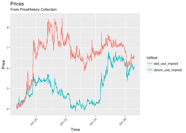
Step 4 - Add a second dataset
We can add a additional datesets to our line plot with another geom_line entry. You can add as many as you want but be mindful of the axis scale and the overall readability. You don't want your charts to be too busy.
ggplot(prices, aes(timestamp))+
# red sbd_usd_implied line
  geom_line(aes(x=timestamp, y=sbd_usd_implied, colour="sbd_usd_implied"))+
# blue steem_usd_implied line
  geom_line(aes(x=timestamp, y=steem_usd_implied, colour="steem_usd_implied"))+
# axis label adjustments
  theme(axis.text.x = element_text(angle=45, hjust=1)) +
# titles and labels
  labs(x="Time", y="Price", title="Prices", subtitle="From
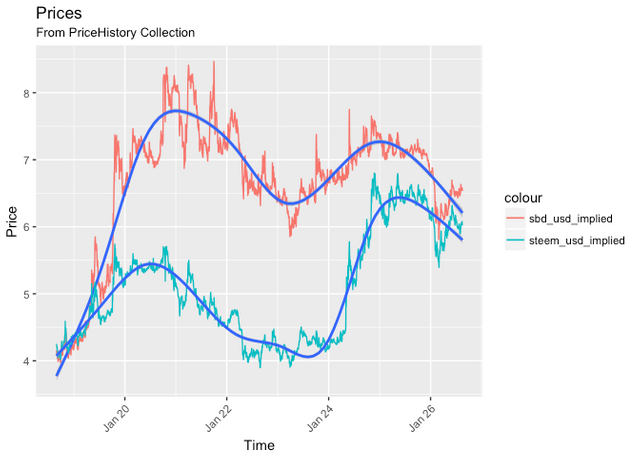
Step 5 - Adding a moving average or trend line
With high fidelity or very granular data it can be difficult to discern the overall movement or trend. A moving average line can help emphasize this. ggplot makes this easy.
ggplot(prices)+
  geom_line(aes(x=timestamp, y=sbd_usd_implied, colour="sbd_usd_implied"))+
# smoothed moving average line
  geom_smooth(aes(x=timestamp, y=sbd_usd_implied))+
# smoothed moving average line
  geom_line(aes(x=timestamp, y=steem_usd_implied, colour="steem_usd_implied"))+
  geom_smooth(aes(x=timestamp, y=steem_usd_implied))+
  theme(axis.text.x = element_text(angle=45, hjust=1)) +
  labs(x="Time", y="Price", title="Prices", subtitle="From PriceHistory Collection")
Let's make it Pretty!
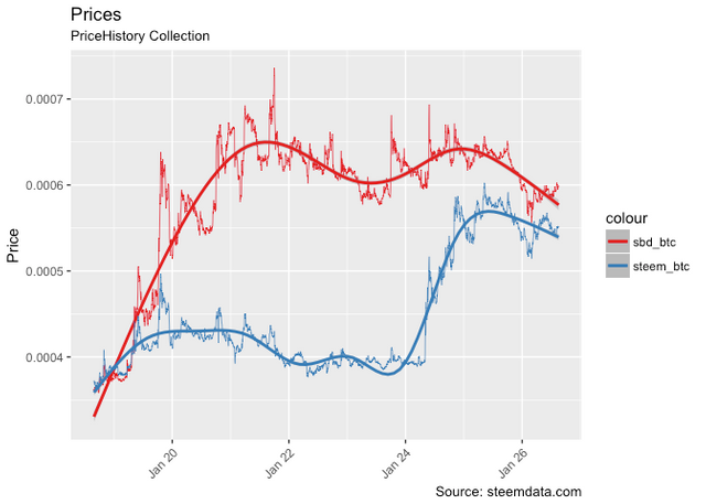
Step 6 - Beautifying our plots
ColorBrewer palettes are used commonly by graphic designers in their infographics. Thanfully we can use them in R too. In the RStudio console, try these commands
> ?RColorBrewer
> display.brewer.all()
You can paste this code into your R Script file and run it to render your plot with the new ColorBrewer palette. Note, we have a slightly less ugly red and blue.
# load ColorBrewer palettes
library(RColorBrewer)
ggplot(prices)+
# select a palette by name. Set1 in this case.
  scale_colour_brewer(palette = "Set1")+
  geom_line(aes(x=timestamp, y=sbd_btc, colour="sbd_btc"), size=0.25)+
  geom_smooth(aes(x=timestamp, y=sbd_btc, colour="sbd_btc"), size=1)+
  geom_line(aes(x=timestamp, y=steem_btc, colour="steem_btc"), size=0.25)+
  geom_smooth(aes(x=timestamp, y=steem_btc, colour="steem_btc"), size=1)+
  theme(axis.text.x = element_text(angle=45, hjust=1)) +
  labs(x=NULL, y="Price",
       title="Prices",
       subtitle="PriceHistory Collection",
       caption="Source: steemdata.com")
Lets Theme!
Step 7 - Customizing pre-canned themes
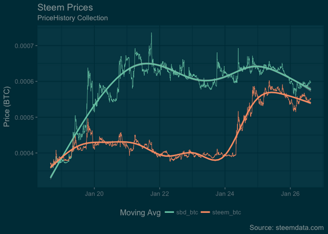
The ggthemes library offers numerous starting points for customization. We'll start with a nice dark one called solarized2 that uses the well known solarized palette.
We'll also have a first attempt at customizing the legend to make better use of the plot canvas.
library(ggthemes)
ggplot(prices)+
  # Pre-canned theme from lib ggthemes
  theme_solarized_2(light = FALSE) +
  # Plot sbd_btc
  geom_line(aes(x=timestamp, y=sbd_btc, colour="sbd_btc"), size=0.25)+
  # Plot smoothed moving avg for SBD
  geom_smooth(aes(x=timestamp, y=sbd_btc, colour="sbd_btc"), size=1)+
  # Plot steem_btc
  geom_line(aes(x=timestamp, y=steem_btc, colour="steem_btc"), size=0.25)+
  # Plot smoothed moving avg for Steem
  geom_smooth(aes(x=timestamp, y=steem_btc, colour="steem_btc"), size=1)+
  # Apply custom labels
  labs(x=NULL, y="Price (BTC)",
       title="Steem Prices", subtitle="PriceHistory Collection",
       caption="Source: steemdata.com")+
  # Move legend to bottom
  theme(legend.position="bottom", legend.box = "horizontal") +
  # Overide legend title and background fill
  guides(color=guide_legend(title="Moving Avg", override.aes=list(fill=NA)))+
  # Use RColourBrewer sets
  scale_colour_brewer("Colors in Set2", palette="Set2")
Looking Good Billy-Ray!
Step 8 - Tweeking meta data and legend labels
It would be nice if we can illustrate the data date range more precisely. This will be important when we have more data and the x-axis becomes harder to discern the exact start and end dates.
This code will extract from our data the max and min dates. Note, this may not be the same ous the data parameters used in our original mongodb query. In our query we asked for all data in January. All that was available was a couple of weeks worth.
# Get the earliest date in the dataset
    startDate <- as.Date(min(prices$timestamp))
# Format the data into something more friendly than an ISO date.
    startDate <- format(startDate, "%a %b %d")
# Repeat for the latest or last date
    endDate <- as.Date(max(prices$timestamp))
    endDate <- format(endDate, "%a %b %d")
We'll also change the legend labels. There are several ways to achieve this but the simplest way is to just rename the columns of our data structure.
# assign data to a new data structure, to avoid messing with our raw original data
    newPrices <- prices
# give each column new names
    names(newPrices) <- c("timestamp", "BTC/USD", "STEEM/BTC", "SBD/BTC", "STEEM/SDB", "STEEM/USD", "SBD/USD")
Now we can go ahead and plot.
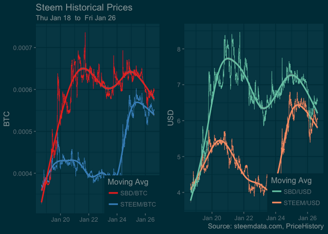
In this example we create a second plot using two more columns from our data structure. I've chosen to put them on a different plot because they have different units of measure (BTC vs USD). I've also used a different color palette to make this distinction more obvious.
Putting them on the same plot will be misleading and too busy. You can try it and see what I mean.
I've assigned each plot to an object (p and q). We can then pass these objects to the gridExtra function which will put them into a panel plot of one row and two columns.
library(gridExtra)
q <- ggplot(newPrices)+
  theme_solarized_2(light = FALSE) +
  geom_line(aes(x=timestamp, y=`STEEM/BTC`, colour="STEEM/BTC"), size=0.25)+
  geom_smooth(aes(x=timestamp, y=`STEEM/BTC`, colour="STEEM/BTC"), size=1)+
  geom_line(aes(x=timestamp, y=`SBD/BTC`, colour="SBD/BTC"), size=0.25)+
  geom_smooth(aes(x=timestamp, y=`SBD/BTC`, colour="SBD/BTC"), size=1)+
  labs(x=NULL, y="BTC", title="Steem Historical Prices", subtitle=paste(startDate," to ", endDate), caption=" ")+
  theme(legend.position="bottom", legend.box = "horizontal") +
  guides(color=guide_legend(title="Moving Avg", override.aes=list(fill=NA)))+
  theme(legend.justification=c(1,0), legend.position=c(1,0))+
  scale_colour_brewer("Colors in Set1", palette="Set1")
p <- ggplot(newPrices)+
  theme_solarized_2(light = FALSE) +
  geom_line(aes(x=timestamp, y=`STEEM/USD`, colour="STEEM/USD"), size=0.25)+
  geom_smooth(aes(x=timestamp, y=`STEEM/USD`, colour="STEEM/USD"), size=1)+
  geom_line(aes(x=timestamp, y=`SBD/USD`, colour="SBD/USD"), size=0.25)+
  geom_smooth(aes(x=timestamp, y=`SBD/USD`, colour="SBD/USD"), size=1)+
  labs(x=NULL, y="USD", title=" ", subtitle=" ", caption="Source: steemdata.com, PriceHistory")+
  theme(legend.position="bottom", legend.box = "horizontal") +
  guides(color=guide_legend(title="Moving Avg", override.aes=list(fill=NA)))+
  theme(legend.justification=c(1,0), legend.position=c(1,0))+
  scale_colour_brewer("Colors in Set2", palette="Set2")
grid.arrange(q,p, ncol=2)
Behold our Panel Plots

Posted on Utopian.io - Rewarding Open Source Contributors
So detailed. Thank you for taking the time to present it.
@originalworks
Thank you for the contribution. It has been approved.
You can contact us on Discord.
[utopian-moderator]
Hey @morningtundra I am @utopian-io. I have just upvoted you!
Achievements
Suggestions
Get Noticed!
Community-Driven Witness!
I am the first and only Steem Community-Driven Witness. Participate on Discord. Lets GROW TOGETHER!
Up-vote this comment to grow my power and help Open Source contributions like this one. Want to chat? Join me on Discord https://discord.gg/Pc8HG9x