I thought for this weekend I would have a little fun and show you one of my recent projects.

My wife and I were recently looking to purchase a car. Things are pretty tight now and with a baby on the way we needed to get something that was both affordable and low maintenance. We decided on the following criteria:

less than 150000 miles
Between $1000-$4000
Made in the year 2000 or newer
No/minimal repairs needed

There were lots of good choices so I decided to make a spreadsheet! Anyone who knows me will tell you that I probably spend more time making spreadsheets than I do actually saving time with those sheets... That may or may not be true but either way, I love making spreadsheets!

https://xkcd.com/1908/

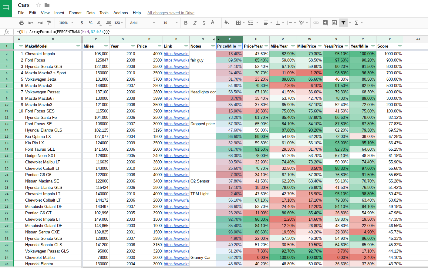
Here is what I came up with

https://docs.google.com/spreadsheets/d/1Ahxb_8m3sbBa_WazRrDAFs74wnRwQ5t4RVLFzqPKnwc/edit#gid=0

The goal of this sheet was to find out how good of a (relative) deal each car was. The better the deal, the more I would want to buy it right?

If you don't care how it works and just want to use it, skip to the bottom.

Lets start with columns B-G. These columns are simply where we input our data. Make/Model, Miles, Year, Price, Link, and notes. (I took out the links because they give out a lot of information about me.... so yeah...).

So what I did was every time I found a car that met our criteria, I put it's information on the sheet. I ended up with quite a few options which is good because the more options I have, the better my data will be.

Alright, lets get complicated! So the next thing I wanted to do was to see how much each car should be worth based on all the other cars. So in column H I calculated how much the car should cost based on it's mileage. The formula I used is one that I discovered while building this spreadsheet, "TREND".

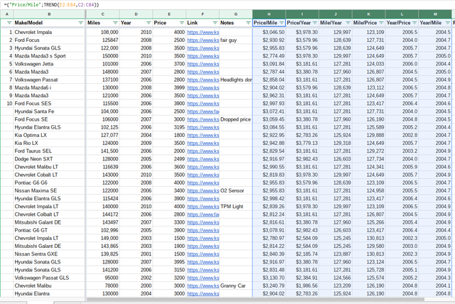
TREND is a formula that finds the "line of best fit" using the "least squares method." Basically that means that we could graph all of the cars' mileage vs their price and draw a line that is as close to all the points as possible. Then, it looks at the mileage and calculates what the price should be if it was right on that trend line.

So my formula looks like this ={"Price/Mile";TREND(E2:E84,C2:C84)}

let me break it down real quick

{"Price/Mile";} -- is just to make a header at the top of the column
TREND(E2:E84 -- trend is the formula, it looks at column E which is the price
C2:C84) -- looking at column C which is the Mileage

The formula returns the expected price based on mileage in column C

Columns I-N are all similar, they show the expected price/mile/year based on the trend lines

Column H: Price/Mile
Column I: Price/Year
Column J:Mile/Year
Column K:Mile/Price
Column L:Year/Price
Column M:Year/Mile

This shows what the price, year, and miles should be of each car based on the trend line of all the cars. (I hope that makes sense...)

Next up we have column N-S. These columns show how far off the expected results are from the actual.

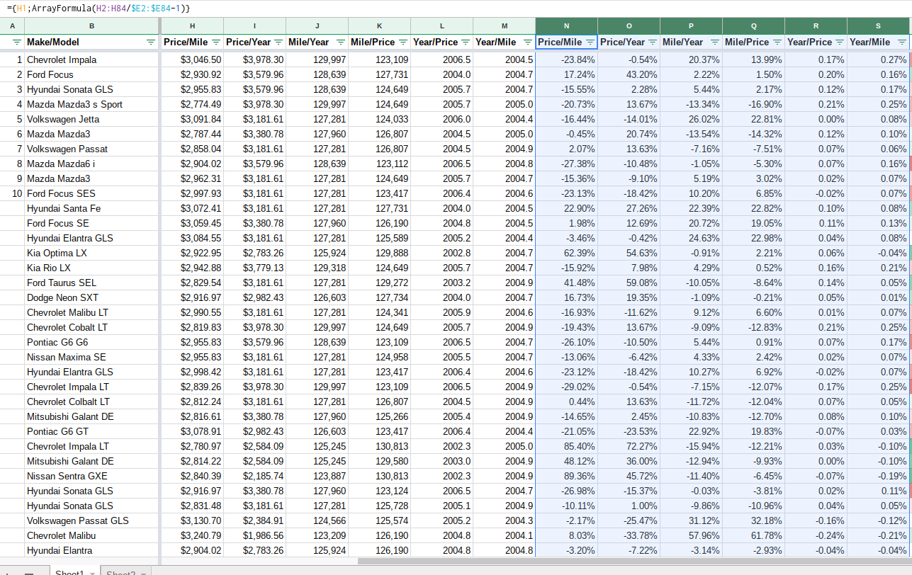
They all have the same basic formula: ={H1;ArrayFormula(H2:H84/$E2:$E84-1)}

{H1;} -- Again, this is for the header column, it will show "H1" which is "Price/Mile"
Arrayformula( -- Array formulas allow you to type one formula and it fills in multiple cells. That's all I'll say about that for now.
H2:H84/$E2:$E84 -- taking column H (which is our expected price based on mileage) and dividing it by column E (which is our actual price)
-1 -- I get the -1 at the end because I am using a simplified version of the ROI calculation which is (gain from investment - cost of investment) / cost of investment. This formula can be simplified to Gain from investment / cost of investment - 1. So my expected price is my "gain" and my actual price is my "cost" because I pay the actual amount but if it is worth more than that I am getting a positive ROI.

Each of these column run a similar calculation.

Columns T-Y compare the ROI's in each of the columns N-S to see which gives the best and which give the worst. I calculate this with the "Percentrank" formula: ={N1; ArrayFormula(PERCENTRANK(N:N,N2:N84))}

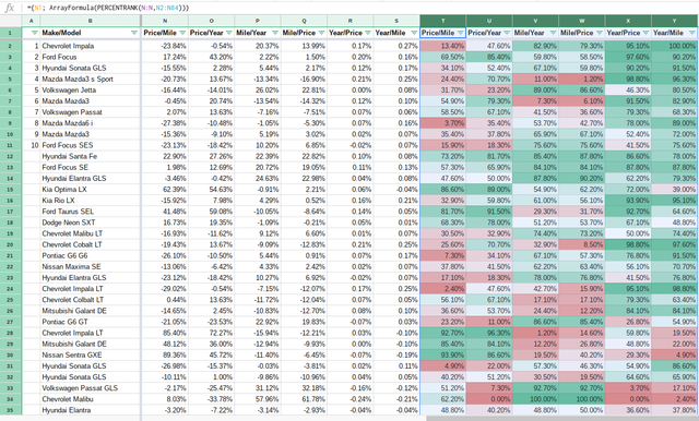
{N1;} -- this is getting the header again from column N "Price/Mile"
Percentrant(N:N,N2:N84) -- this gives you the percentile of each roi in column N. In other words, the highest ROI would be 100% and the lowest would be 0%. The middle one would be 50% and everything else would fall in between.

The rest of the columns have a similar calculation

Column Z gives us the final score. It takes the average of columns T-Y. This shows how good of a deal each vehicle is compared to all the others. It also has a few other things in that formula but we will get to that in a bit.

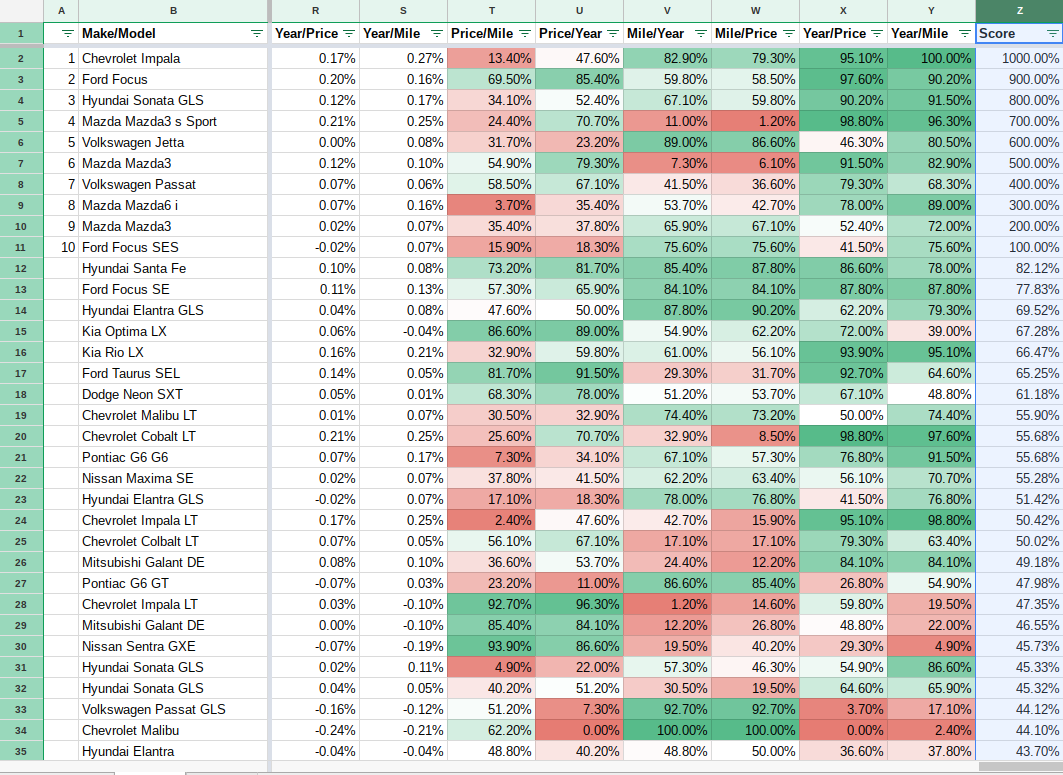
Now that we calculated all of that, we can sort column z from biggest to smallest and it will show us the cars that are the best deals at the top. So what I did at this point was my wife and I looked through the top half of the cars (~30) and ruled out any that we (she) didn't like. We would type "No" in column A for any cars that we weren't interested in. Then we picked our top 10 and put them in order from our favorite to our least favorite. We wrote these numbers in column A with 1 being our favorite and 2 our second and so on.

Column Z has this formula: =if(A2="No",-100,if(A2>=1,11-A2, AVERAGE(T2:Y2)))

You can't do an array formula with "average" so I had to put this formula in every cell in column Z using autofill
if(A2="No",-100, -- this is a simple "if" formula. If A2 has "No" in it, show -100, otherwise...
if(A2>=1,11-A2, -- another "if" formula. If A2 is greater than or equal to 1 (because it is in the top 10), 11-A2. This makes our top choice the biggest number (11-1=10, 11-2=9, etc).If it doesn't have a number in it...
AVERAGE(T2:Y2) -- this gives us our score as the average of T-Y

I then set up appointments to meet with our top three choices and we ended up going with the Ford Focus. Hopefully it will work out well for us and the baby!

Shortcomings

There are a few things that could make this more accurate.

1. The "least square method" is only a straight line, it could be more accurate if there was a formula that could do more powerful regressions. This would make our trend line more accurate
2. This method does not take make/model into account. I couldn't think of a good way to do it but if you could weight higher quality cars more than lower quality cars that would of course make this more accurate.
3. The sample size is fairly small. Obviously if we could have more cars we could have a better sample to get the trend lines but these are all the cars in my local area I could find. Maybe if you had more historical information it could be better

All in all, I think it works good enough to be an interesting tool to help you decide what car to buy. Don't take it as gospel, just an analytical tool.

If you don't care how it works, you just want to know how to use it

1. Go to my spreadsheet and click File->make a copy...
2. Input any cars that fit your critera into columns B-G
3. Sort column Z from biggest to smallest
4. The top cars are the best deals and you can look at columns T-Y for what things make it a better or worst deal. (Green=Above Average, Red=Below Average; the darker, the further from the average)
5. You can move cars to the bottom by typing "No" in column A and re-sorting column Z
6. You can move cars to the top by typing a number(1-10) in column A (the smaller the number, the closer to the top).

Let me know what you think! Are there ways to improve this? Did I miss something? Is this totally unnecessary and I'm just a crazy nerd?

I have many more spreadsheets I could share if you're interested. Let me know which ones you want to hear about.

Time management
Budget
Cash Flow Management (Debt paydown and bills calculator)
Cryptocurrency Trading
Secret Santa autogenerator
Family Savings and Loan (P2P lending and borrowing within my family)
Timecards
Chore sheet (allows people to choose what chores they want to do with the prices slowly going up until someone does them)

I think that's about it! Be sure to upvote and follow! Keep the comments coming!